
- What is Dividends ? and How do They Work | Everything You Need to Know | Expert’s Top Picks
- Interest Rate Risk – How to Mitigate the Risk | A Complete Guide For Beginners
- What Is Capital Budgeting and Cash Flow in Finance Management?
- Treynor Measure Vs Sharpe Measure
- Binomial Option Pricing Model
- What is Financial Risk and Its Types?
- The Most In-demand and Highest Paying Jobs in Canada

Binomial Option Pricing Model
Last updated on 30th Sep 2020, Artciles, Blog, Investment Banking
The binomial option pricing model is an options valuation method developed in 1979. The binomial option pricing model uses an iterative procedure, allowing for the specification of nodes, or points in time, during the time span between the valuation date and the option’s expiration date.
As per the binomial option pricing model, the price of an option is equal to the difference between the present value of the stock (as computed through a binomial tree) and the spot price.
- The binomial option pricing model values options using an iterative approach utilizing multiple periods to value American options.
- With the model, there are two possible outcomes with each iteration—a move up or a move down that follow a binomial tree.
- The model is intuitive and is used more frequently in practice than the well-known Black-Scholes model.
Subscribe For Free Demo
Error: Contact form not found.
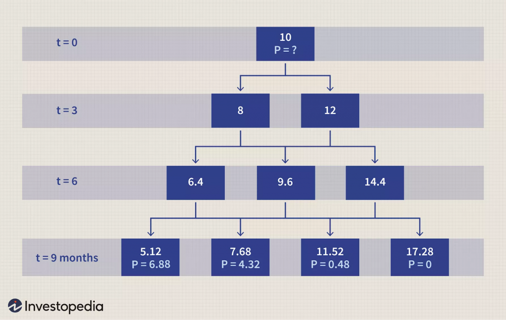
The model reduces possibilities of price changes and removes the possibility for arbitrage. A simplified example of a binomial tree might look something like this:
Basics of the Binomial Option Pricing Model
With binomial option price models, the assumptions are that there are two possible outcomes, hence the binomial part of the model. With a pricing model, the two outcomes are a move up, or a move down. The major advantage to a binomial option pricing model is that they’re mathematically simple. Yet these models can become complex in a multi-period model.
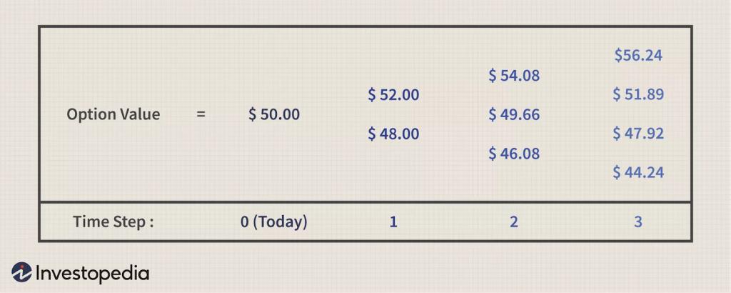
In contrast to the Black-Scholes model, which provides a numerical result based on inputs, the binomial model allows for the calculation of the asset and the option for multiple periods along with the range of possible results for each period (see below).
The advantage of this multi-period view is that the user can visualize the change in asset price from period to period and evaluate the option based on decisions made at different points in time. For a U.S-based option, which can be exercised at any time before the expiration date, the binomial model can provide insight as to when exercising the option may be advisable and when it should be held for longer periods. By looking at the binomial tree of values, a trader can determine in advance when a decision on an exercise may occur. If the option has a positive value, there is the possibility of exercise whereas, if the option has a value less than zero, it should be held for longer periods.
Calculating Price with the Binomial Model
The basic method of calculating the binomial option model is to use the same probability each period for success and failure until the option expires. However, a trader can incorporate different probabilities for each period based on new information obtained as time passes.
A binomial tree is a useful tool when pricing American options and embedded options. Its simplicity is its advantage and disadvantage at the same time. The tree is easy to model out mechanically, but the problem lies in the possible values the underlying asset can take in one period. In a binomial tree model, the underlying asset can only be worth exactly one of two possible values, which is not realistic, as assets can be worth any number of values within any given range.
For example,
There may be a 50/50 chance that the underlying asset price can increase or decrease by 30 percent in one period. For the second period, however, the probability that the underlying asset price will increase may grow to 70/30.

Enroll in CAPM Certification Course & Get Noticed By Top Hiring Companies
Weekday / Weekend BatchesSee Batch DetailsAnother example,
If an investor is evaluating an oil well, that investor is not sure what the value of that oil well is, but there is a 50/50 chance that the price will go up. If oil prices go up in Period 1 making the oil well more valuable and the market fundamentals now point to continued increases in oil prices, the probability of further appreciation in price may now be 70 percent. The binomial model allows for this flexibility; the Black-Scholes model does not.
Real World Example of Binomial Option Pricing Model
A simplified example of a binomial tree has only one step. Assume there is a stock that is priced at $100 per share. In one month, the price of this stock will go up by $10 or go down by $10, creating this situation:
- Stock price = $100
- Stock price in one month (up state) = $110
- Stock price in one month (down state) = $90
Next, assume there is a call option available on this stock that expires in one month and has a strike price of $100. In the up state, this call option is worth $10, and in the down state, it is worth $0. The binomial model can calculate what the price of the call option should be today.
For simplification purposes, assume that an investor purchases one-half share of stock and writes or sells one call option. The total investment today is the price of half a share less the price of the option, and the possible payoffs at the end of the month are:
- Cost today = $50 – option price
- Portfolio value (up state) = $55 – max ($110 – $100, 0) = $45
- Portfolio value (down state) = $45 – max($90 – $100, 0) = $45
The portfolio payoff is equal no matter how the stock price moves. Given this outcome, assuming no arbitrage opportunities, an investor should earn the risk-free rate over the course of the month. The cost today must be equal to the payoff discounted at the risk-free rate for one month. The equation to solve is thus:
- Option price = $50 – $45 x e ^ (-risk-free rate x T), where e is the mathematical constant 2.7183.
Assuming the risk-free rate is 3% per year, and T equals 0.0833 (one divided by 12), then the price of the call option today is $5.11.
Due to its simple and iterative structure, the binomial option pricing model presents certain unique advantages. For example, since it provides a stream of valuations for a derivative for each node in a span of time, it is useful for valuing derivatives such as American options—which can be executed anytime between the purchase date and expiration date. It is also much simpler than other pricing models such as the Black-Scholes model.