
- Probability Density Function in Statistics Tutorial | Definition, Formula & Examples
- Best Clojure Tutorial | Ultimate Guide to Learn [UPDATED]
- Introduction to RapidMiner Tutorial | Get Started with RapidMiner
- R Tutorial
- Spark SQL Tutorial
- Data Extraction in R Tutorial
- Introduction to RapidMiner Tutorial | Get Started with RapidMiner
- Data Scientist vs Data Analyst vs Data Engineer Tutorial
- Unsupervised Learning with Clustering- Machine Learning Tutorial
- Data Scientist Report 2020 Tutorial
- Tutorial on Statistics and Probability for Data Science | All you need to know [ OverView ]
- Machine Learning-K-Means Clustering Algorithm Tutorial
- Julia Tutorial
- Data Science Tutorial

Probability Density Function in Statistics Tutorial | Definition, Formula & Examples
Last updated on 26th Oct 2022, Blog, Data Science, Tutorials
What exactly is the Probability Density Function and How Does It Work?
In statistics, a Probability Density Function (PDF) is a function that, by defining the relationship between a random variable and its probability in such a way that you can find the probability of the variable by using the function, it is possible to determine the probability of the random variable.A probability density function, also known as a PDF, is a statistical expression that defines a probability distribution, or the likelihood of an outcome, for a discrete random variable, such as a stock or an exchange-traded fund (ETF). A continuous random variable, on the other hand, is considered to have an infinite number of possible outcomes. A discrete random variable is distinct from a continuous random variable in that it is possible to provide an exact value for the variable.
They can be divided mostly into two categories:
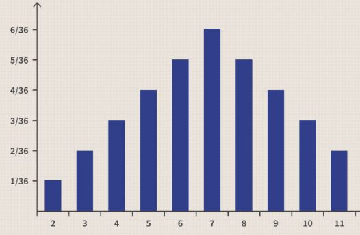
Discrete Variable: A discrete variable is a variable that can only take on a certain finite value inside a specific range. Discrete variables can only take on a value between 0 and 1. The values are typically separated by a definite gap, such as the sum of two dice in this example. When two dice are rolled and the totals of those rolls are added together, the result can only be a number that falls within a range that does not exceed 12 (as the maximum result of a dice throw is 6). Additionally, the values are unquestionable.
A continuous variable: is a random variable that can take on an unlimited number of possible values within a given range of values. One example of a continuous variable is the quantity of rainfall that occurs in a given month. The amount of rain that was measured could be 1.7 centimetres, although the precise measurement is unknown. It is possible for it to be 1.701, 1.7687, and other values as well. As a consequence of this, all you can do is declare the value range it inhabits. It is possible for it to take on an unlimited number of different values while remaining inside this value.
How Do You Locate the Probability Density Function When Working with Statistics?
The following are the three most important steps:
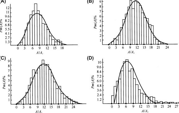
Converting the data into discrete form by plotting it as a histogram is the first step in the process of using a histogram to summarise the density. A graph with categorical values along the x-axis and bins of varying heights, known as a histogram, can provide you with a count of the values that fall into a particular category. The number of bins is an essential variable since it establishes both the total number of bars in the histogram and the width of each bar. This will tell you how the density of your data will be plotted.
Estimation of the parametric density being Carried Out A PDF can be formatted to seem like a variety of different common functions. You will be able to determine the sort of function that it is by looking at the form of the histogram. To obtain our density, you can figure it out by calculating the parameters connected with the function. You can do the following to see if or not our histogram is an excellent fit for the function:
- 1.Plot the density function and evaluate the shape of the histograms.
- 2.Examine hypothetical examples of the function alongside real-world examples.
- 3.Use a statistical test.
Calculating Non-Parametric Density Estimates In situations in which the shape of the histogram does not match a common probability density function, or cannot be made to fit one, you calculate the density by using all of the samples in the data and applying certain algorithms. This is known as performing non-parametric density estimation. The Kernel Density Estimation is an example of one of these algorithms. It does this by calculating and smoothing the probabilities with the use of a mathematical function so that their sum is always 1. In order to accomplish this, you will require the following parameters:
- 1.The smoothing parameter for the bandwidth is as follows: Sets the total number of samples that are utilised to calculate an estimate of the probability of a new point being created.
- 2.Helps to maintain control over the overall sample distribution. Basis Function.
History:
According to the Probability density hypothesis, a Probability density work (PDF), also known as the density of a constant arbitrary variable, is a capability whose value at some random example (or point) in the example space (the arrangement of potential qualities taken by the irregular variable) can be interpreted as giving a relative probability that the worth of the irregular variable would be near that sample. In other words, the PDF measures the density of a constant arbitrary variable.
At the end of the day, even though the outright probability for a consistent arbitrary variable to take on a specific worth is 0 (since there is an endless arrangement of potential qualities in any case), the value of the PDF at two unique examples can be utilised to figure out, in a specific draw of the arbitrary variable. This can be done by comparing the values of the PDF.
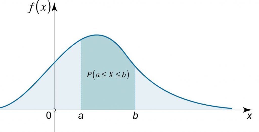
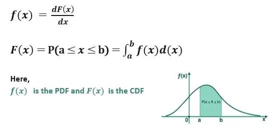
In a more precise sense, the PDF is used to determine the Probability density of an arbitrary variable falling within a particular scope of characteristics, as opposed to taking on anyone’s worth. This is done rather than taking on anyone’s worth. This probability density is given by the indispensable of this current variable’s PDF over that range; more specifically, In other words, it is given by the region under the density work. The probability density work is positive everywhere, and its basic value across the entire space is equal to one. This is true despite the fact that the space itself is nonnegative.
There have also been instances where the terms “Probability density dispersion function” and “Probability density function” have been used to refer to the Probability density work. However, the use of this term is not typical among those who work with probability and analysts. It is possible that “Probability density circulation work” will be used in some other sources when the Probability density conveyance will be described as a capacity over various combinations of qualities, or it may refer to the total dispersion capacity, or it may be a Probability density mass capacity (PMF) rather than the density. Further confounding matters is the fact that the term “density work” can also be used to refer to the probability density mass capacity. In general, the PMF is used when dealing with discrete irregular factors (which are arbitrary factors that take values on a countable set), and the PDF is used when dealing with constant irregular factors.
KEY TAKEAWAYS:
- Probability density functions are a type of statistical analysis that can be utilised to evaluate the likelihood of a certain result for a discrete value (e.g., the price of a stock or ETF).
- PDFs are usually plotted on a graph that looks like a bell curve, with the probability of the outcomes falling below the curve in the graph.
- While it is possible to precisely measure a discrete variable, continuous variables can take on an endless number of values.
- PDFs are a useful tool for determining the possible risk and benefit of investing in a specific security or fund within a portfolio.
- The bell-shaped curve that results from the normal distribution is frequently used as an illustration.
In comparison to a CDF, what is a PDF?
- A probability density function, also known as a PDF, is a function that provides an explanation of which values are likely to appear in a process that generates data at any given moment or for any given draw.A cumulative distribution function, or CDF, instead illustrates.
- how these marginal probabilities add together to reach a total of one hundred percent (or 5.0) of the potential outcomes. We are able to determine the likelihood, with the help of a CDF, that the result of a variable will be greater than or equal to a certain anticipated value.
What exactly is a function?
- At its most fundamental level, a function can be conceptualised as a container that accepts input and produces output in response to that input. In the great majority of circumstances, the function must actually carry out some action in conjunction with the input in order for the result to be of any use.
- Let’s define our own function. Let’s imagine that this function accepts a number as its input, adds 2 to the number that was given as its input, and then returns the new number as its output. Graphically, our function is represented (in the form of a box)
Density of the Probabilities:
- A probability distribution p is associated with the random variable x. (x).
- The probability density, also referred to simply as the density, is the term used to describe the relationship that exists between the outcomes of a random variable and its associated probability.
- If the value of a random variable is continuous, then the probability can be determined using a tool called the probability density function, or PDF for short.
- The probability distribution is the shape of the probability density function across the domain for a random variable, and common probability distributions have names like “uniform,” “normal,” and “exponential,” amongst others. The probability distribution can also be thought of as the probability density function.
- We are interested in the density of the probability associated with a random variable that we have been given.
- For instance, if we have a random sample of a variable, we might be interested in learning several properties, such as the shape of the probability distribution, the value that is most likely to occur, the range of possible values, and so on.
- The moments of a probability distribution, such as the mean and the variance, can be calculated with the help of the probability distribution for a random variable.
- However, knowing the probability distribution for a random variable can also be helpful for other, more general considerations, such as determining whether an observation is unlikely or very unlikely and whether it could be an outlier or an anomaly.
- The issue is that we could not be aware of the probability distribution associated with a random variable.
- Because we don’t have access to all of the possible outcomes for a random variable, knowing the distribution of a random variable is extremely rare.
- In point of fact, all we have at our disposal is a selection of different observations. As a result of this, we are required to choose a probability distribution.
- This problem is known as probability density estimation, or just “density estimation” for short, because we are using the observations in a random sample to estimate the overall density of probabilities that extends beyond just the sample of data that we have available.
The procedure of estimating the density of a random variable will take you through a few different steps:
- The first thing that has to be done is to use a straightforward histogram to examine the distribution of data throughout the random sample.
- We might be able to find a widespread and well-understood probability distribution that can be utilised by looking at the histogram.
- One example of this would be the normal distribution. In the event that this is not the case, we might have to fit a model in order to estimate the distribution.
In the following sections, we will examine each of these steps in further detail before moving on to the next one:
For the sake of simplicity, we will concentrate on univariate data, also known as data with one random variable. Although these processes can be applied to multivariate data, it is possible that they will become more difficult to complete as the number of variables in the data set grows.
Conclusion:
The term “probability distributions” is frequently used incorrectly to refer to probability density functions. This leads to confusion due to the fact that they are, in reality, two different things: probability density functions apply to continuous variables, whereas probability distributions apply to discrete variables; probability density functions return probability densities, whereas probability distribution functions return probabilities; and, according to the definition of probability density functions, separate outcomes have zero probabilities. When it comes to probability distributions, individual outcomes can have probabilities that are not zero.