How to Create a Project Plan in Excel?

When should you use Excel for project management?

Should you stick with Excel, or spring for project management software?

It’s a tough question — on one hand, you risk being stuck in the middle of a project with a tool that lacks the advanced features needed to properly execute daily tasks, while on the other hand, you may spend thousands of dollars on software that’s more powerful than you need it to be.

When Excel is the best choice?

Sometimes less is more. Just because you can purchase fancy project management software platforms out there doesn’t mean you should open up your wallet. Here are a few reasons to eschew those solutions for Excel:

• You’re a one-man band: If you’re, say, a small contractor firm consisting of just yourself or a couple of others, you don’t need a platform that’s loaded with features and geared toward large enterprise firms.
• You just want something easy: Even the easiest-to-use project management software platforms have a learning curve. With Excel, you just punch in your task list, materials orders, man-hours, or whatever else you want to track right in the spreadsheet.
• You want to save money: Good software is expensive, costing hundreds or even thousands of dollars per month. That money comes directly from your bottom line, so if Excel meets your needs, you can save a lot of money simply by declining to get specialized software.

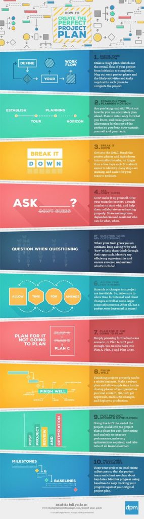
How To Create The Perfect Project Plan In 10 Steps

Now let’s learn how to make a project plan—one that works in harmony with the way we manage projects in the 21st century.

We’ve created this project management plan checklist as a handy guide to creating a project plan for any project. Whether it’s a large cake, a large website platform, or even something non-digital, the principles and steps are the same.

Here’s an infographic summary of the steps. Read on for detailed explanations below.

How to Create a Project Plan in Excel

I am often asked by people how they can create a project plan without any project software. While I always say investing in good project management software makes sense if you have to create lots of project plans sometimes if you need to quickly create a plan then Microsoft Excel can be used. What I set out below is how you can create a project plan in Excel however you can do similar steps in other spreadsheet software such as Apple Numbers and Google Sheets. The last step however is how to how to add a Gantt chart to the plan and only applies to Microsoft Excel.

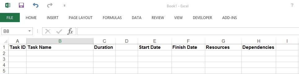
Step One – Create Basic Plan Layout

The first thing to do is open a blank Microsoft Excel workbook and across the top of sheet 1 write at the top:

• Column A Task ID
• Column B Task Name
• Column C Duration
• Column D (Leave blank for the moment)
• Column E Start Date
• Column F Finish Date
• Column G Resources
• Column H Dependencies
• You should have something that looks like this

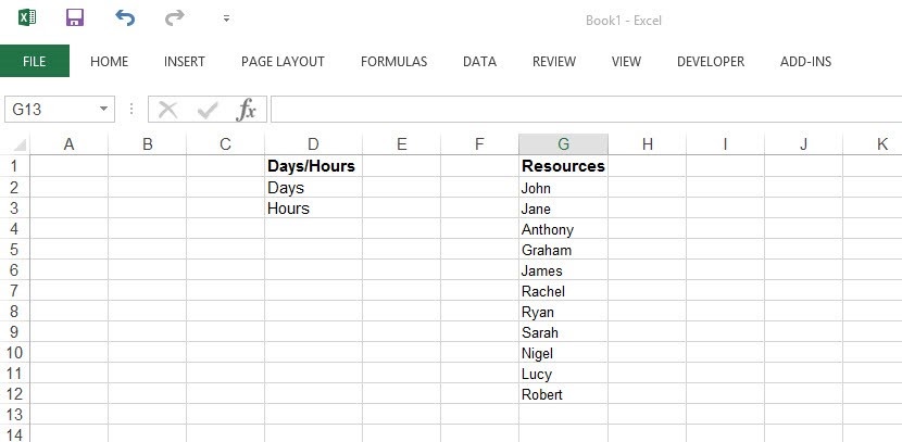
Step Two – How to create a list for duration and resources

The next step is to create your drop down lists for columns D and G. To do this click on Sheet 2. At the top of column D on sheet 2 write Days/Hours. Then in the cell directly below the one you have just populated write Days. After that in the cell underneath where you have written Days write Hours.

With days and hours complete move over to column G and at the top write Resources. Under where you have written resources on each cell directly below write the names of each person who is going to work on your project. When you have completed inputting all the names you should have one person on each row. That is sheet 2 complete and it should look like this.

Step Three – How to switch all tasks from hours to days with one click

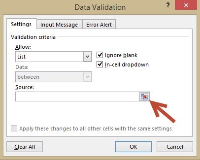
Go back to sheet 1 as you are now going to create the dropdown lists. At the top of Column D (which you left blank in step one) click on the cell and then click on the Data tab in the ribbon followed by clicking on Data Validation. Doing this brings up the data validation dialog box and you need to click the drop down arrow in the Allow section.

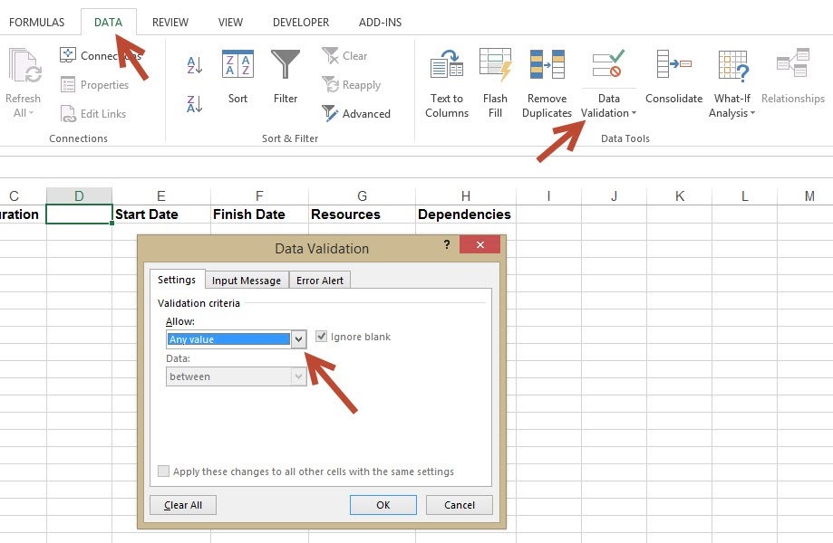
When you click this button a drop down appears and you need to click List. Once you have done this a new section appears called Source. Click on the button at the end of the source section.

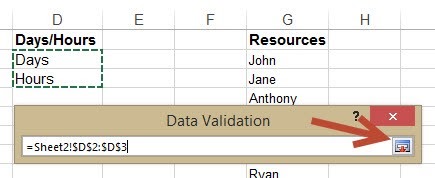
The Data Validation box will become smaller and at this point click on sheet 2. When you are on sheet 2 click cell D2 and without releasing the mouse button drag down to cell D3. You should see the Data Validation populated like the picture below, if it is then click the button at the end of the box and then click ok. You now have on sheet 1 a drop down in column D which is days or hours.

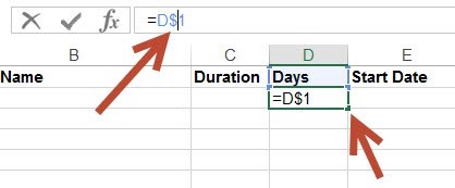
On sheet 1 click on Cell D2 and press = and then click on Cell D1 followed by enter. What this does is set Cell D2 to be the same as D1. Once you have done this click inside the formula bar between D and 1. In here you need to enter the dollar sign $. The final part of step three is to click the bottom right of Cell D2 and it down to cell D100.

Step Four – How to add resource name dropdown list

This step is a repeat of step 3 but this time it is the resources column. Directly underneath where you have written Resources click on the cell and without releasing the mouse button drag down to cell G100. Then as before click on the Data tab in the ribbon followed by clicking on Data Validation. Doing this brings up the data validation dialog box and you need to click the drop down arrow in the Allow section. When you click this button a drop down appears and you need to click List. Once you have done this a new section appears called Source. Click on the button at the end of the source section.

The Data Validation box will become smaller and at this point click on sheet 2. When you are on sheet 2 click cell G2 and without releasing the mouse button drag down to the last cell you have populated with a name. You should see the Data Validation populated like before, if it is then click the button at the end of the box and then click ok. You now have on sheet 1 a drop down in all of the cells of column G below the resources title.

Step Five – How to add a calendar date picker for start and finish

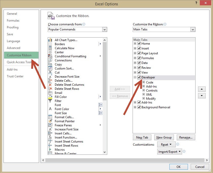
The next step is to create a calendar drop down for the start and finish columns. To do this you need to have the developer tab available on the ribbon. If you do not have it click File and then Options. From here click Customize Ribbon, then tick the Developer check box and press Ok.

When you go back to sheet 1 you should see the developer tab on the ribbon next to view. Click the Developer tab followed by Insert. This brings up a drop down list and you need to select the Custom option which is the image of a screwdriver and spanner.

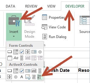
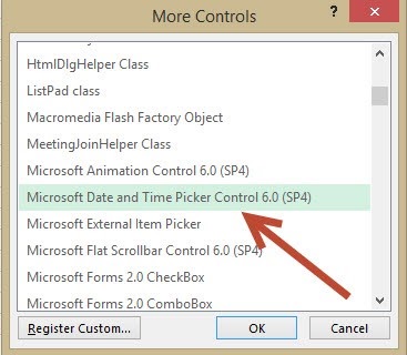
This brings up a pop up; from here scroll down select Microsoft Date and Time Picker Control and click OK.

Once you have clicked ok you will go back to sheet 1 and your cursor would have changed to a cross. Click the top left of cell E2 and while still holding down the mouse drag it to the bottom right hand corner of the cell. This draws a box and inside you will find it populated with a date. You may have to resize the row height and column width so you can make the box bigger to display the date clearly. The last thing to do is right click on the date box you have just made and click Copy.

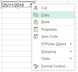
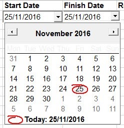
Then right click on cell F2 and select Paste. You should now find you have a date box in the finish column. Repeat this by pasting a date box in as many rows as you need for tasks in your plan and then when you are down click on the deign mode button in the ribbon. Now when you click the drop down arrow you should see a calendar where you can choose your date.

Step Six – How to create sub tasks

To make it easier to manage tasks you can break them down into sub tasks and then roll up all the sub tasks into the main task. The first thing to do is create a list like below. Make sure you keep the duration blank for Task 1 for the moment

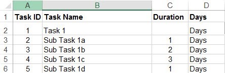
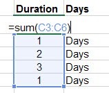
Next click on cell C2, press = and type sum(C3:C6). This will add up all the sub tasks to give a total for task 1. Should you need to adjust any of the sub tasks durations then this will automatically update the top level task.

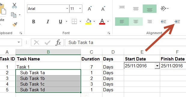
To make it easier to read the plan sub tasks can be indented. Select all the task name cells you want to indent and click the Indent button; see image below which show the indent button.

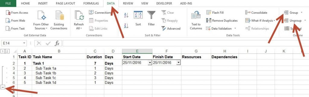
Finally sub tasks can be grouped together which enables them to be minimised. This is useful when tasks have been completed so you can just see the top level task. To do this click on the Data ribbon and then select the rows you want to group by clicking on the row numbers (in this example rows 3,4,5 and 6). With all the rows selected click Group and a bar appears to the far left of the spreadsheet. Click the Minus sign on this bar will hide your sub tasks. To display them again just click on the minus again. If you which to remove the group just select the rows again and click Ungroup.

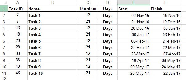
Step Seven – Create a table for the Gantt chart

With your working plan created you can also create a Gantt chart of the high level tasks that you can share with your project stakeholders. To do this add a third sheet and click on sheet 3. Create a table similar to what you created before in step 1 but only include the high level tasks. There is no need to create the dropdowns or the calendar in this table. Populate your table with information from sheet 1 (dates and duration) See the image below.

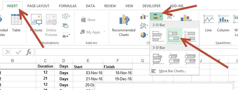
Step Eight – Create the Gantt chart

With the table created to start to create your Gantt chart you need to select Insert from the ribbon and then select the Second 2-D Bar Graph from the horizontal graph button.

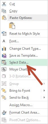
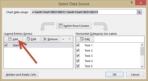
A blank square will then appear on the spreadsheet and you need to right click on this square. On the menu that pops up click Select Data.

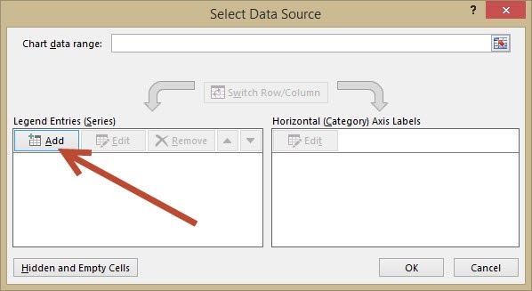
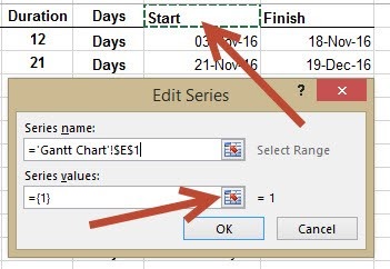
This will bring up the select data source dialog box and on this box you need to click Add.

This will open the edit series dialog box and when it does click on Start. Doing this will place a dotted green line around the start cell. Once you have done this click the button next to = 1 on the edit series dialog box.

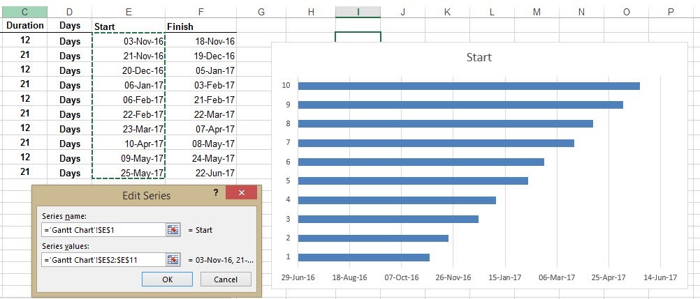
This minimises the edit series dialog box and you need to click the first date in the start column and without letting go of the mouse drag it down to the last date. Once you have done this click the button at the end of the edit series box.

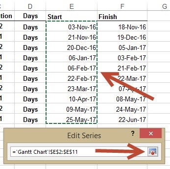
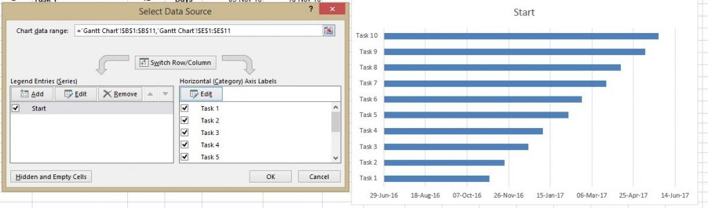
You should now have a graph that looks like the image below. If so click the Ok button to close the edit series dialog box.

The next step is to format the axis so it displays the names of the tasks. To do this right click on the graph again and choose Select Data source as before. This time when the select data source dialog box appears select Edit.

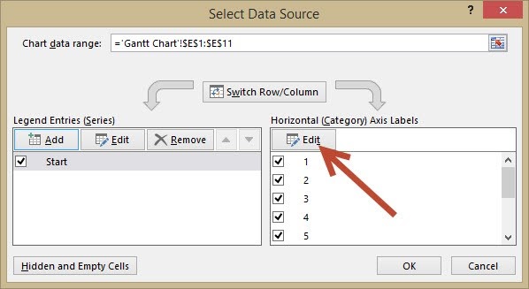
Clicking this brings up the axis labels dialog box and here you want to click the button next to select range.

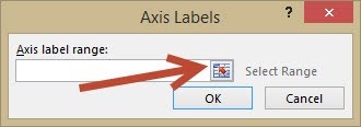
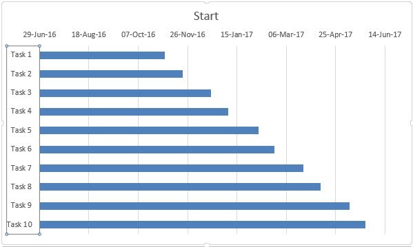
As you did before for the dates click on the first task and drag down to the last task. A green dotted line will appear round all the selected tasks. Click on the axis labels button.

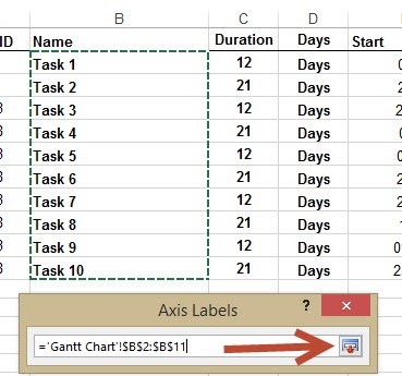
This will add the task names to the graph, however for a Gantt chart the graph is upside down so the next stage is to reverse the order of the tasks.

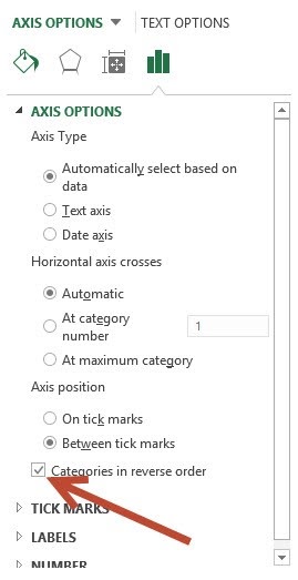
To reverse the order of the tasks right click on the graph and select Format Axis from the menu that appears.

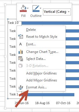
Doing this brings up the axis options and you need to scroll down to the axis position and check the box that says Categories in reverse order.

As you can see if your graph is the same as the image below it is starting to look like a Gantt chart. However rather than start dates you want to show duration of the tasks.

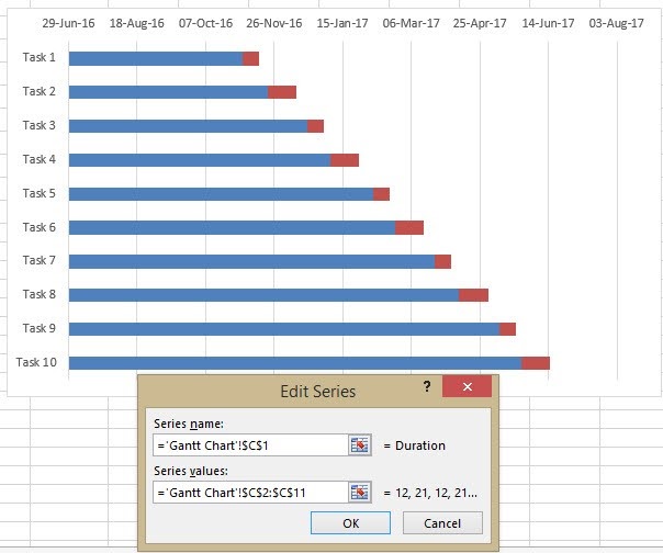
Once again right click on the graph and choose Select Data Source. When the dialog box appears again you need to click Add.

Following the same steps as before click the cell at the top but this time choose duration. Doing this will place a dotted green line around the duration cell. Once you have done this click the button next to = 1 on the edit series dialog box. This minimises the edit series dialog box and you need to click the first number in the duration column and without letting go of the mouse drag it down to the last number. Once you have done this click the button at the end of the edit series box. You graph should now look like the image below.

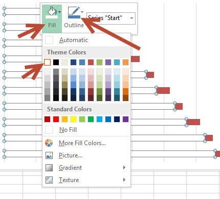
The final stage is to make it look like a Gantt chart by hiding the bars before the start of the task. To hide them move your mouse over one of the bars you want to hide and right click. Doing this pops up a menu and from here you need to select Fill and choose white (same as background). Once you have done this choose Outline and select no outline.

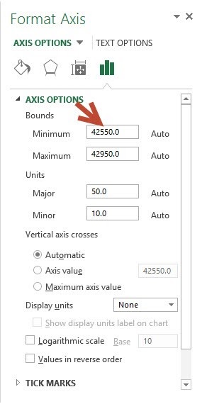
Congratulations you now have a Gantt chart. However there are a couple of things you can do to make it look better. Again right click on the Gantt chart and select Format Axis like you did before. This time you need to click the Three Bars and the area you want to look at is the Bounds section. Changing the Minimum will move the chart to the left removing the white space that you now have.

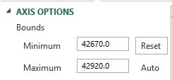
It is the third and fourth digits that needing changing. In my case I changed the 55 to 67 and this moved the chart to where I wanted it. The numbers maybe slightly different for you. Have a go and change these two digits until you get the chart exactly where you want it. If it all goes wrong just hit Reset and it will move back to before you changed the numbers. This will take a little bit of trial and error to get right.

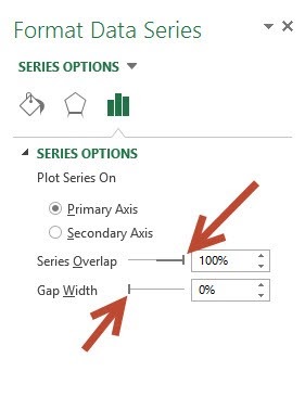
Next with the Gantt chart positioned over to the left you can now make the bars look a bit better. To do this right click on the duration bars and choose Format Data Series.

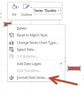
Again click on the Three Bars but this time scroll down to the Series Overlap and Gap Width. Set the series overlap to 100% and gap width to 0%. This will make the bars closer together and look more like a Gantt chart.

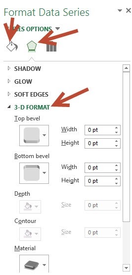
Still within the format data series options you can click on the Fill and Shape button to change the colour and appearance of the bars.

By the end you should have a Gantt chart that look like the image below.

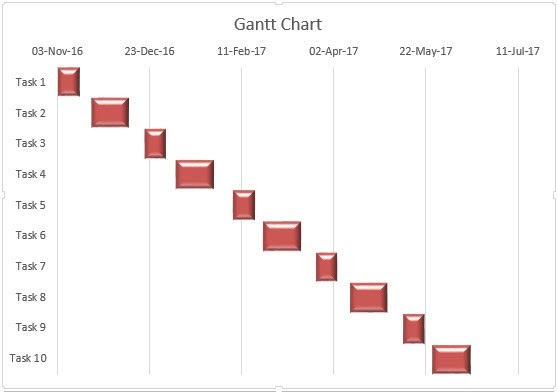
That is the end of the complete tutorial on how to create a project plan with a Gantt chart in Excel. Well done for getting all the way through, I hope you have found this useful and can now create excellent project plans in Excel.