MS Excel Tutorial

Microsoft Excel is one of the most used software applications of all time. Hundreds of millions of people around the world use Microsoft Excel. You can use Excel to enter all sorts of data and perform financial, mathematical or statistical calculations.

1.Range:

A range in Excel is a collection of two or more cells. This chapter gives an overview of some very important range operations.

2.Formulas and Functions:

A formula is an expression which calculates the value of a cell. Functions are predefined formulas and are already available in Excel.

Microsoft Excel is a commercial spreadsheet application, written and distributed by Microsoft for Microsoft Windows and Mac OS X. At the time of writing this tutorial the Microsoft excel version was 2010 for Microsoft Windows and 2011 for Mac OS X.

Microsoft Excel is a spreadsheet tool capable of performing calculations, analyzing data and integrating information from different programs.

By default, documents saved in Excel 2010 are saved with the .xlsx extension whereas the file extension of the prior Excel versions are .xls.

This tutorial has been designed for computer users who would like to learn Microsoft Excel in easy and simple steps. It will be highly useful for those learners who do not have prior exposure to Microsoft applications.

Prerequisites

Before proceeding with this tutorial, you should have a basic understanding of Computer peripherals like mouse, keyboard, monitor, screen etc. and their basic operations. You should also have the basic skills of file management and folder navigations.

BASIC EXCEL SKILLS :

Now a days, any job requires basic Excel skills. These basic Excel skills are – familiarity with Excel ribbons & UI, ability to enter and format data, calculate totals & summaries thru formulas, highlight data that meets certain conditions, creating simple reports & charts, understanding the importance of keyboard shortcuts & productivity tricks. Based on my experience of training more than 5,000 students in various online & physical training programs, the following 6 areas form the core of basic Excel skills.

GETTING STARTED :

Excel is a massive application with 1000s of features and 100s of ribbon (menu) commands. It is very easy to get lost once you open Excel. So one of the basic survival skills is to understand how to navigate Excel and access the features you are looking for.

1. Quick Access Toolbar:

This is a place where all the important tools can be placed. When you start Excel for the very first time, it has only 3 icons (Save, Undo, Redo). But you can add any feature of Excel to to Quick Access Toolbar so that you can easily access it from anywhere (hence the name).

2. Ribbon:

 Ribbon is like an expanded menu. It depicts all the features of Excel in easy to understand form. Since Excel has 1000s of features, they are grouped in to several ribbons. The most important ribbons are – Home, Insert, Formulas, Page Layout & Data.

3. Formula Bar:

This is where any calculations or formulas you write will appear. You will understand the relevance of it once you start building formulas.

4. Spreadsheet Grid:

 This is where all your numbers, data, charts & drawings will go. Each Excel file can contain several sheets. But the spreadsheet grid shows few rows & columns of active spreadsheet. To see more rows or columns you can use the scroll bars to the left or at bottom. If you want to access other sheets, just click on the sheet name (or use the shortcut CTRL+Page Up or CTRL+Page Down).

5. Status bar: 

This tells us what is going on with Excel at any time. You can tell if Excel is busy calculating a formula, creating a pivot report or recording a macro by just looking at the status bar. The status bar also shows quick summaries of selected cells (count, sum, average, minimum or maximum values). You can change this by right clicking on it and choosing which summaries to show.

ENTERING & FORMATTING DATA, NUMBERS & TABLES :

Handling Data would be one of the main reasons why you are using Excel. Excel is quite intuitive and simple to use when it comes to typing data or handling it. Because of its grid nature, it can store & manage thousands of data points with ease.Built in features like copy, paste, find, highlight, go to, styles etc. make the process of maintaining data very easy for you.

Functions :

Discover how functions in Excel help you save time. If you are new to functions in Excel, we recommend you to read our introduction to Formulas and Functions first.

1.Count and Sum:

The most used functions in Excel are the functions that count and sum. You can count and sum based on one criteria or multiple criteria.

2.Logical:

Learn how to use Excel’s logical functions, such as IF, AND, OR and NOT.

3.Cell References:

Cell references in Excel are very important. Understand the difference between relative, absolute and mixed reference, and you are on your way to success.

4.Date & Time:

To enter a date in Excel, use the “/” or “-” characters. To enter a time, use the “:” (colon).

5.Text:

Excel has many functions to offer when it comes to manipulating text strings.

6.Lookup & Reference:

Learn all about Excel’s lookup & reference functions, such as VLOOKUP, HLOOKUP, MATCH, INDEX and CHOOSE.

7.Financial:

This chapter illustrates Excel’s most popular financial functions.

8.Statistical:

An overview of some very useful statistical functions in Excel.

9.Round:

This chapter illustrates three functions to round numbers in Excel. ROUND, ROUNDUP and ROUNDDOWN.

10.Formula Errors:

This chapter teaches you how to deal with some common formula errors in Excel.

11.Array Formulas:

This chapter helps you understand array formulas in Excel. Single cell array formulas perform multiple calculations in one cell.

Data Analysis :

This section illustrates the powerful features Excel has to offer to analyze data.

1.Sort:

You can sort your Excel data on one column or multiple columns. You can sort in ascending or descending order.

2.Filter:

Filter your Excel data if you only want to display records that meet certain criteria.

3.Conditional Formatting:

Conditional formatting in Excel enables you to highlight cells with a certain color, depending on the cell’s value.

4.Charts:

A simple Excel chart can say more than a sheet full of numbers. As you’ll see, creating charts is very easy.

5.Pivot Tables:

Pivot tables are one of Excel’s most powerful features. A pivot table allows you to extract the significance from a large, detailed data set.

6.Tables:

Tables allow you to analyze your data in Excel quickly and easily.

7.What-If Analysis:

What-If Analysis in Excel allows you to try out different values (scenarios) for formulas.

8.Solver:

Excel includes a tool called solver that uses techniques from the operations research to find optimal solutions for all kind of decision problems.

9.Analysis ToolPak:

The Analysis ToolPak is an Excel add-in program that provides data analysis tools for financial, statistical and engineering data analysis.

WHY LEARN EXCEL?

Analysts, consultants, marketing professionals, bankers, and accountants all use Excel on a consistent basis. You might even find that other random professionals like graphic designers and engineers are working away with the powerful formulas and charts that come with Excel.

Seeing as how Excel is so prominent in the workforce, it pays to learn all about it and put that experience on your resume. You might find that your current degree isn’t yielding any job prospects, so getting into Excel could get you a job in the meantime.

EXCEL TUTORIALS : BEGINNER TO ADVANCED :

The following links describe a set of excel tutorials which are useful for learning basic, intermediate and advanced MS Excel. It includes tutorials about useful excel functions, excel macros, excel charts, excel dashboard, Infographics with Excel. It also covers how to apply most of the important mathematical and statistical techniques with Excel.

Entering Text and Numbers :

Microsoft Excel is an electronic spreadsheet that runs on a personal computer. You can use it to organize your data into rows and columns. You can also use it to perform mathematical calculations quickly. This tutorial teaches Microsoft Excel basics. Although knowledge of how to navigate in a Windows environment is helpful, this tutorial was created for the computer novice. This lesson will introduce you to the Excel window. You use the window to interact with Excel.

Entering Excel Formulas and Formatting Data :

Familiarized you with the Excel 2007 window, taught you how to move around the window, and how to enter data. A major strength of Excel is that you can perform mathematical calculations and format your data. In this lesson, you learn how to perform basic mathematical calculations and how to format text and numerical data.

Creating Excel Functions, Filling Cells, and Printing :

By using functions, you can quickly and easily make many useful calculations, such as finding an average, the highest number, the lowest number, and a count of the number of items in a list. Microsoft Excel has many functions you can use. You can also use Microsoft Excel to fill cells automatically with a series.For example, you can have Excel automatically fill your worksheet with days of the week, months of the year, years, or other types of series.

A header is text that appears at the top of every page of your printed worksheet. A footer is text that appears at the bottom of every page of your printed worksheet. You can use a header or footer to display among other things titles, page numbers, or logos. Once you have completed your Excel worksheet, you may want to print it. This lesson teaches you how to use functions, how to create a series, how to create headers and footers, and how to print.

How to Move Between Cells :

Since a workbook in Excel contains cells rather than open space on a blank page, movement while typing is a bit different than Microsoft Word. You can use the arrow keys to move around or click directly in cells.

Here are other keyboard keys you can use:

• TAB – move one cell to the right
• SHIFT + TAB – Move one cell to the left
• ENTER – Move to the beginning of the next row
• SHIFT + ENTER – Move to the cell directly above the current one, in the previous row

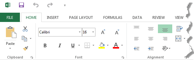
User Interface :

The setup of Excel is straightforward if you learn how to use it, and you will see that it is very similar to other software in Microsoft Office. When you open a workbook, the top bar of tools is called the ribbon, the different categories along the top of the ribbon are tabs.

You will utilize the Home tab the most. Most of the tool groups on the ribbon also have a small arrow in the bottom right-hand corner that you can click to expand the customization of each tool.

When you begin typing in a cell on the spreadsheet (a cell is one of the boxes where a column and row meet), it will display the text on the sheet and in the formula bar located at the top of the spreadsheet. You can make edits in either of these locations.

Printing :

A vertical, dotted line indicates the printing section of the sheet. Adjust column widths to help move all your data into this section. To print, select the File tab and Print. It will show a preview of the page. The barrier lines that were on the sheet do not show on the preview; you must add borders to create separation, if needed.

How to Find a Total Using SUM :

The fastest way to find the total of a group of numbers is to use AutoSum. The AutoSum tool is under the Formulas tab or the Home tab. To use it, click the cell where you want the total to show (best placed in line with the amounts being added). Then, hit AutoSum to fill in the formula and total automatically. After you hit AutoSum, you can change the exact range of cells used in the total by clicking and dragging on the highlight box of cells. Hit the ENTER key.

10 Tips for Making the Most of Excel

After learning all these skills, use these 10 helpful tips to help you make the most out of Excel. Microsoft Excel can save you a lot of time on projects, but only if you know some of these tricks.

1. Quick Analysis :

The Quick Analysis tool shows up when you highlight a range of cells. It is a small box to the lower right of the highlighted area. It has numerous quick-use tools and allows you to view a preview of each change when you hover over it with the mouse. Some of the tools Quick Analysis provides are conditional formatting, chart creation, automatic total calculations, tables, and sparklines.

When you use Quick Analysis, it saves the time it takes to go through tabs finding the right tools to make big changes like this. Of course, for more customization, you may want to take the harder route, but Quick Analysis speeds things up.

2. Filter :

The Filter is something we talked about earlier in this reading that can really help you to find certain items or groups of items from a large group of data. We had used the Sort & Filter button, but you can use the Filter button on the Data tab instead. When you turn on the Filter, it adds arrowed drop-down menus on all sections of the data, which you can use to pull up list items from a certain category or by other criteria.

3. Control Keys :

When you normally use the arrow keys in a worksheet on Excel, they move the selection around to different cells. However, this can waste time if you must arrow all the way down a sheet to the right cell you want. To move around faster, hold down the CTRL key, and then hit the arrows. Now, the selection jumps through sections of data quickly.

4. Adjust Column Widths in Excel :

When you adjust the width of a column, you can click and drag on the barrier line between two columns. However, the faster way to do this is by double-clicking on that line. The cells in that column will automatically adjust to fit the contents. You can do the same with the rows.

To adjust all the columns and rows at once, click the arrow in the top left corner of the sheet so that everything selected, then double-click in the same spot between two columns. Now, everything will automatically adjust so that you do not have to manually change the widths of every column and row in the worksheet.

5. Flash Fill and AutoFill in Excel :

Flash Fill is a feature that comes in handy when you make a list. If you have typed the list before in the spreadsheet, when you begin to type the first word, it will show you a suggestion for a flash fill of the rest of the list. Press ENTER to accept the Flash Fill suggestion.

6. Absolute Cell Reference :

An absolute cell reference keeps a referred cell in place when using a formula. What that means is, when you enter a formula using two cells in the equation, you can make one “absolute” to make sure that it does not shift when you copy the formula to multiple cells. You can make either part of the cell reference absolute or the whole thing (row and column). Learn more about this in the Cell References section above.

7. Transpose Tables in Microsoft Excel :

When you transpose tables in Excel, you reverse the rows and columns. To transpose a table, select a range, right-click on it, and hit copy. Go to a blank area on the spreadsheet and right-click. Hit Paste Special. A box of options will come up, where you can click the box for “Transpose”. Click OK, and the data will flip itself in the new cells.

8. Text to Columns :

When you want to copy a list to a spreadsheet in Excel, this is what you can do to make sure all the elements of the list have a designated spot.

In the Convert Text to Columns Wizard that appears, make sure these settings are selected: Delimited, Tab, Comma (select this according to what is separating your list currently – commas, semicolons, or spaces), General. Then, Finish. The items on the list should now have their places on the sheet.

9. Inserting a Screenshot :

Rather than going to another window, hitting the print screen button on your keyboard, then pasting it into the sheet on Excel, you can use the Screenshot tool. On the Insert tab, find the Screenshot button and select the window you want to paste a screenshot from; it will paste itself in your worksheet.

10. Show Formulas :

To get a better visual of all the current formulas used in the spreadsheet, press Ctrl + ~. Press the keys again to hide the formulas.

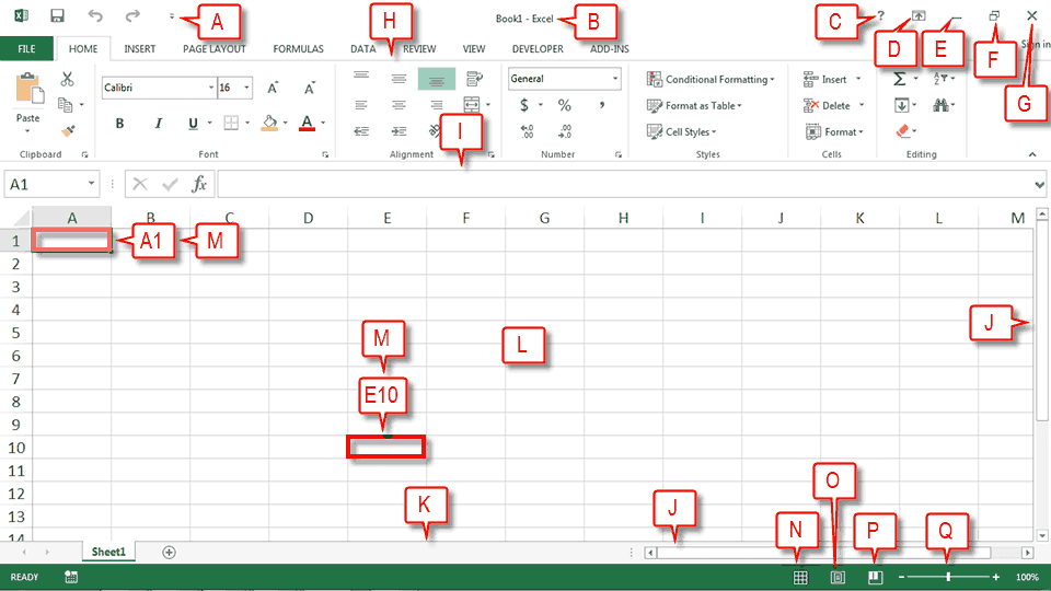
When you open an Excel worksheet, you are presented with the Excel window. You use this window to interact with the software—you type your data into the window and you use the window to tell Excel what to do. In this section, I will explain the parts of the Excel window.

A.Quick Access Toolbar:

In the upper-left corner of the window is the Quick Access toolbar, sometimes referred to as the QAT. The Quick Access Toolbar provides commands you frequently use. Save, Undo, and Redo appear on the toolbar by default. Click Save to save your file, Undo to roll back an action you have taken, and Redo to reapply an action you have rolled back.

B.Title Bar:

In the top center of the window to the right of the Quick Access toolbar is the Title bar. The Title Bar displays the title of your workbook. Excel names the first new workbook you open Book1. As you open additional new workbooks, Excel names them sequentially. When you save a workbook, you assign the workbook a new name.

C.Help Button:

The Help button, along with several other buttons, is located in the upper-right corner of the window. It takes you to the Excel help area. In the help area, you can search for information on how to perform tasks.

D.Ribbon Display Options Button :

\The Ribbon Display Options button is located next to the Help button. Use it to display the following menu options: Auto-hide Ribbon, Show Tabs, and Show Tabs and Commands. To learn more about these options, see the section The Excel Ribbon.

E.Minimize Button :

The Minimize button is located next to the Ribbon Display Options button. To remove Excel from view and place the Excel icon on the Windows taskbar, click the Minimize button. To restore Excel, click the Excel icon on the Windows taskbar.

F.Restore Down :

The Restore Down button is located next to the Minimize button. The Restore Down button reduces the size of the Excel window. When you click the Restore Down button, it turns into the Maximize button.

Maximize Button:

The Maximize button fills your screen with the Excel window. When you click the Maximize button, it turns into the Restore Down button.

G.Close Button :

The Close button is located in the far right corner of the Excel window. It closes the active workbook. When you click the Close button, if you have not previously saved your workbook or if you have made changes to your workbook since you last saved, a dialog box opens. Click Save if you want to save your changes, Don’t Save if you do not want to save your changes, or Cancel if you have decided not to close your workbook. If the workbook you are closing is the only workbook open, the Close button also closes Excel.

H.Ribbon:

To tell software what to do, you issue commands. In Excel, you can use the Ribbon to issue commands. The Ribbon is located below the Title bar. To learn more about the Ribbon, see the section The Excel Ribbon.

I.Formula Bar:

Optionally, the Formula Bar is found below the Ribbon. Use the Formula Bar to enter and edit data. If your Formula Bar is not visible, follow the steps listed here:

Display the Formula Bar

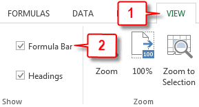
1. 1.Choose the View tab.
2. 2.Click Formula Bar in the Show group. Excel displays the Formula Bar.

J.Vertical and Horizontal Scroll Bars:

You can move up, down, and across your window by dragging the icon located on a scroll bar. The vertical scroll bar is located along the right side of the window. The horizontal scroll bar is located just above the Status bar. To move up and down your worksheet, click and drag the icon on the vertical scroll bar up and down. To move back and forth across your workbook, click and drag the icon on the horizontal scroll bar back and forth.

K.Status Bar:

The Status bar appears at the very bottom of the window and provides information such as the sum, the average, and the count of selected numbers. You can change what displays on the Status bar by right-clicking on the Status bar and selecting the options you want from the Customize Status Bar menu. A check mark next to an item means it is selected. You click an unselected menu item to select it. You click a selected menu item to unselect it.

L.Worksheet:

Just below the Formula Bar is your worksheet. This is where you enter your data. Each worksheet contains columns and rows. The columns are lettered starting with A to Z and then continuing with AA, AB, AC and so on. The rows are numbered starting with one. Only your computer memory and your system resources limit the number of columns and rows you can have in a worksheet.

How to use the worksheet

M Cells: Worksheets are divided into cells. The combination of a column coordinate and a row coordinate make up a cell address. You refer to cells by their cell address. For example, the cell located in the upper left corner of a worksheet is call cell A1, meaning column A, row 1. Column E10 is located under column E on row 10. You enter your data into the cells on the worksheet.

N.Normal Button :

The Normal button formats your worksheet for easy data entry.

O.Page Layout Button :

The Print Layout button displays your workbook in such a way as to make it easy for you to assign printing options and to see how your worksheet will look when printed.

P.Page Break Preview :

The Page Break Preview button displays your workbook and shows where each page begins and ends.

Q.Zoom Slider and Zoom:

The Zoom slider zooms in and out on your workbook. Dragging the slider to the left zooms out, makes your workbook smaller, and allows you to see more of your workbook. Dragging the slider to the right zooms in, makes your workbook larger, and reduces the amount of your workbook you can see. The Zoom slider appears on the Status bar if Zoom Slider is selected on the Status bar menu. The percentage of zoom appears to the right of the zoom slider, if Zoom is selected on the Status bar menu.

Advantages:

1. Sent through Emails

Excel can be sent through email and viewed by most smartphones which makes more convenient .

2. Part of Microsoft Office

Excel is a part of the Microsoft office which comes with most PC, so there is no need to purchase or install it.

3. An All in One Program

Excel is an all in one programme and does not need the addition of financial subsets.

4. Availability of Training Programs and Training Courses

There is training programs and even training courses to make users more familiar with Excel.

5. Secure

Excel files can be password protected for extra security. A user can create a password through Visual Basic programming or directly within the Excel file.[1]

6. Easy connection to OLAP

Excel is capable of connecting directly to OLAP databases and can be integrated in Pivot Tables.

Disadvantages:

1. Viruses

Viruses can be attached to an Excel file through macros. Macros are mini programs that are written into an Excel spread sheet.

2. Slow Execution

Using only one file can make the file size very big and as a result the program might run slowly.

3. Loss of Data

So you might have to break it into smaller files, by doing so there is an increased risk in Excel data being lost.

4. Hard to Use

Although there are training programs, it is still hard to use and some users might not get the hang of it.

5. Space Limit

It limits the number of rows and columns you can use.

Installation

Removing Old or Trial Versions:

Before starting the download of Microsoft Office Professional Plus 2013, you must uninstall any old or trial versions you may still have installed on your machine. Remove the following applications:

• Old or trial versions of Microsoft Office Professional Plus 2013.
• Compatibility Pack for Office 2010.
• Any new versions that you have tried to download/install unsuccessfully.

To remove/uninstall an application:

1. 1.Go to the Control Panel. Depending on the version of Windows you are using, choose one of the following:
   • Add/Remove Programs.
   • Uninstall a program.
2. 2.Locate the application you want to remove.
3. 3.Double-click the application name.
4. 4.Follow the instructions for removing the application.

Downloading pending Windows Updates

Your current operating system (OS) must be up-to-date with Windows Updates before you can install the new software. When the updates are completed, you can install the new software.

To download pending Windows updates:

1. 1.Click the START button.
2. 2.Click ALL PROGRAMS.
3. 3.Click the WINDOWS UPDATE link.
4. 4.Download any pending updates.

32-Bit Versus 64-Bit

Both 32-bit and 64-bit options are available, but we recommend installing the 32-bit version regardless of your OS because the 32-bit option has fewer compatibility issues.

Installation instructions

Create a new workbook

Excel documents are called workbooks. Each workbook contains one or more sheets, typically called spreadsheets. You can add as many sheets as you want to a workbook, or you can create new workbooks to keep your data separate.

When you start excel first time (see the following picture) you can open existing workbook over here or start with a template. Since this is your first time click on the Blank workbook.

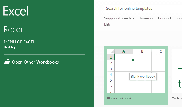
The area down here is where you create your worksheet.

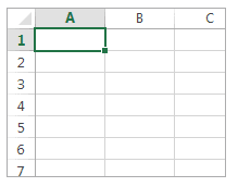
Input your data

• Click an empty cell. For example, cell B2 on the below sheet.
• Type text or a number in the cell.
• Press Enter or Tab to move to the next cell.

Note : Cells are referenced by their location in the row and column on the sheet.

In the following workbook address of 1 is cell B2, 2 is cell B3, and 3 is cell B4.

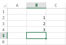
Create a simple formula

Adding numbers is just one of the things you can do, but Excel can do other arithmetical formulas too. Here are some simple formulas to add, subtract, multiply or divide your numbers.

• Move the mouse in a cell and type an equal sign (=). That tells Excel that this cell will contain a formula.
• Type a combination of numbers and calculation operators, like the plus sign (+) for addition, the minus sign (-) for subtraction, the asterisk (*) for multiplication, or the forward slash (/) for the division.
• For example =(6+6*2)/3

• To execute the above formula Press Enter.

Note : To stay on the active cell Press Ctrl+Enter.

Apply a number format

To distinguish between different types of numbers, add a format, like currency, percentages, or dates.

• Select the cells that have numbers you want to format.
• Click Home tab –> General.

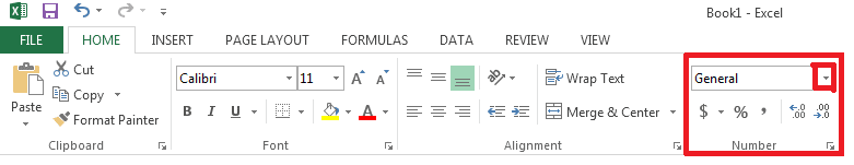
• Pick a number format

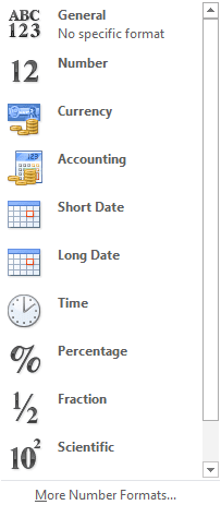
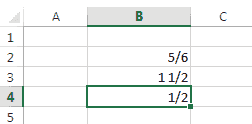
To write fraction number select “fraction”. Here is a sample worksheet with some fraction number.

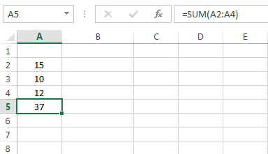
Add your data use AutoSum

When you’ve entered numbers in your sheet, you can add them up to use a fast way that is AutoSum.

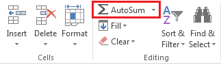
AutoSum adds up the numbers and shows the result in the cell you selected.

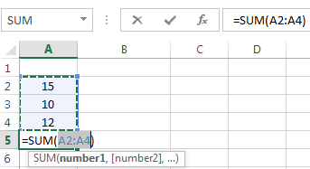
• Press Enter to get desire result.

Put your data in a table

You can store a huge amount of data in a table. That lets you quickly filter or sort your data for starters.

• Select your data by clicking the first cell and dragging to the cell in your data.
  To use the keyboard, hold down Shift while you press the arrow keys to select your data.
• Click the Quick Analysis button in the bottom-right corner of the selection

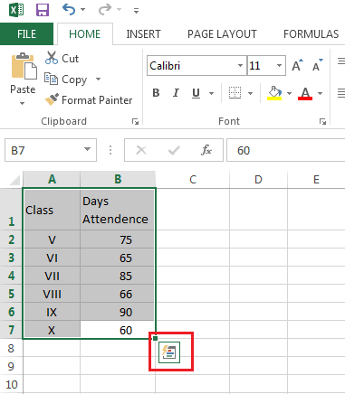
• After clicking Quick Analysis we get the following menu then click on table button.

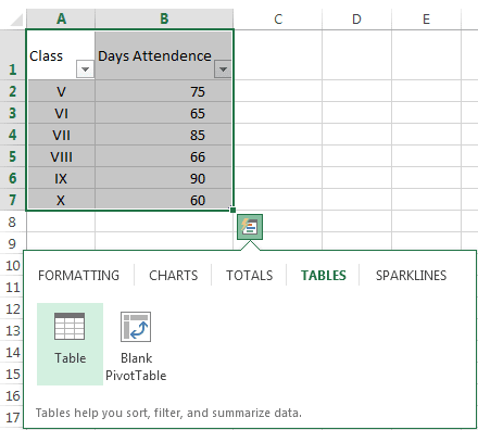
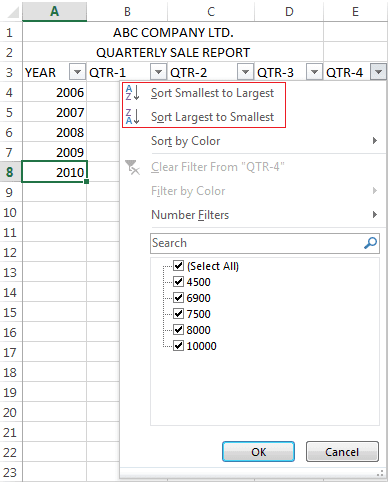
• To filter data, uncheck the Select All box to clear all check marks, and then check the boxes of the data you want to show in your

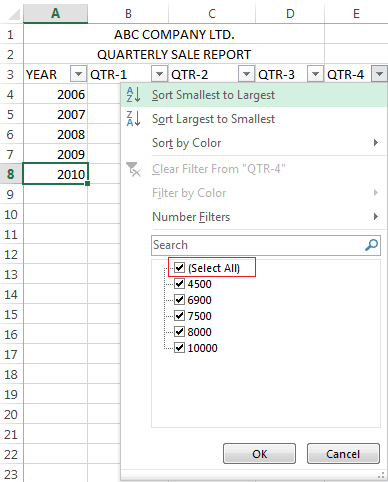
• To sort the data, click Sort A to Z or Sort Z to A.

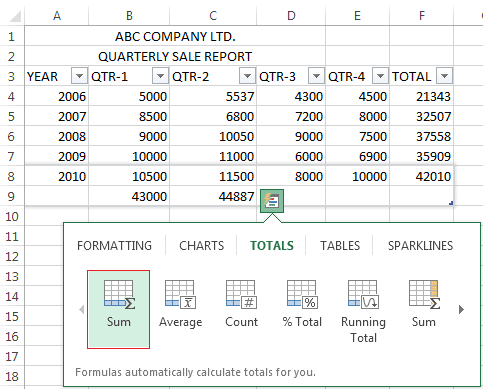
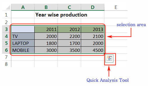
Show totals for your numbers

The Quick Analysis tools let you help to total your numbers quickly, that is the sum, average, or count whatever you want, see the picture below.

• Select the cells which contain numbers which you want to add or count.
• Click the Quick Analysis button in the right-bottom corner of the selection area.
• Then click the Total button or move your cursor across the Total button to see the calculation results for the data.

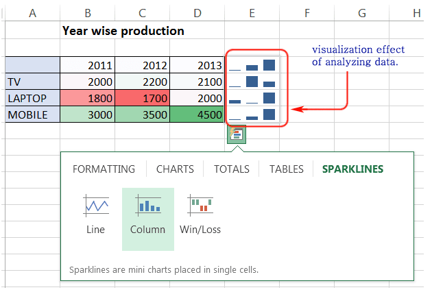
Add meaning to your data

You can see the online preview of your most important data by using conditional formatting or sparklines which highlight your valuable data for better analyzing with visualization. You can use the Quick Analysis tool for a Live Preview to try it out.

Select the data you want for your analyzing.

Click the Quick Analysis button image that appears in the right-bottom corner of your selection, shown in the picture below.

Click on Analysis Tool and get the picture below.

Click on the Formatting tab and get the options shown below.

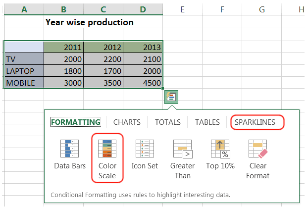
Now pick a color from Color Scale and click Sparklines and move the mouse pointer on the options and get an instant preview, shown below.

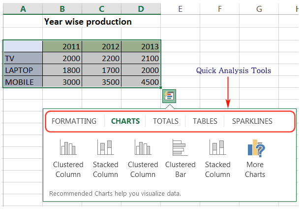
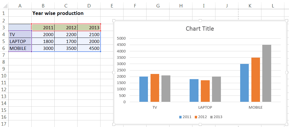
Show your data in a chart

You can use your data to convert into a chart by using Quick Analysis tool for better visual presentation in just a few clicks.

Select your data then quick analysis tool will appear at the right bottom corner of the selection area as shown in the picture below.

Click on Quick Analysis tool then click on Chart and move your mouse pointer on the recommended chart and see which one is your choice. See the picture below.

Click on your choice and the chart will appear in your data sheet as shown below.

Save

To save a file you can use the save button from the Quick Access Toolbar or press Ctrl+S. See the picture below.

You can save the file in another way. Click File — > Save and the following screen will appear.

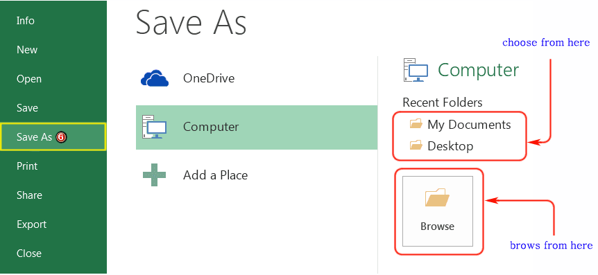
If you are saving the workbook first time the Save As window will appear and you can choose the default showing a folder for saving your workbook otherwise you can browse the folder where you want to save as shown in the above picture. Then in the file name box type the name of the file and click on Save button.

Print

Click the File –> then click Print or press Ctrl+P from the keyboard the preview window will appear.

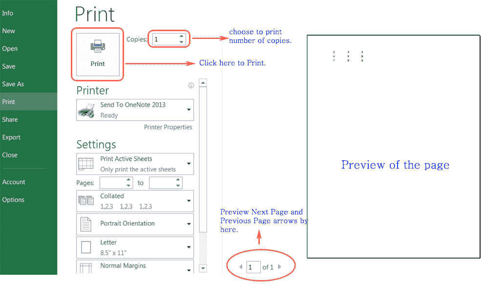
Print preview always appears in black and white format, it depends on the printer setting.

Page setting and printing setting can be changed by using other setting options.

Then click Print to print the page.

Once you have used to the above-mentioned features to organize your data, you can share your work with colleagues and friends in real time, which is yet another fascinating aspect of MS Excel 2013. Using the Excel WebApp, files can be shared and worked upon by others through SkyDrive. Note that if 2 people try to perform the same action on one file simultaneously, you can experience some problems.

Moreover, if someone else is working on a Microsoft Excel worksheet, you cannot open it from SkyDrive on your device. This limitation ensures that there are no conflicting changes in the same file. However, if an Excel file that is stored online is being used by someone, you can (with permission) download or view it. But none of the changes you make will be reflected in the original file which will remain locked unless the other person closes it.

Also remember that the new Excel 2013, like all other applications in Office 2013, automatically saves files to the cloud which you can access through the a browser with the Excel WebApp even if you do not have Excel on your local hard drive.

Moving on in this Excel 2013 lesson, you can even share files via social network direct from Excel 2013. To share your files on networks like Facebook, start by saving them to SkyDrive first. If you haven’t done so, simply click “File” followed by “Share”, and then select “Invite People”. In this way, you will come across “Save As” options in a while.

After this process, you will return back to the Share panel where you see “Post to Social Networks”. You can choose any social network provided that it is linked with your Office 2013 account. Here you can include a message and decide whether others can edit the worksheet you are sharing. After doing this, your post is ready to be shared.