How to use Control Chart Constants?

How to use Control Chart Constants?

CONTROL CHARTS

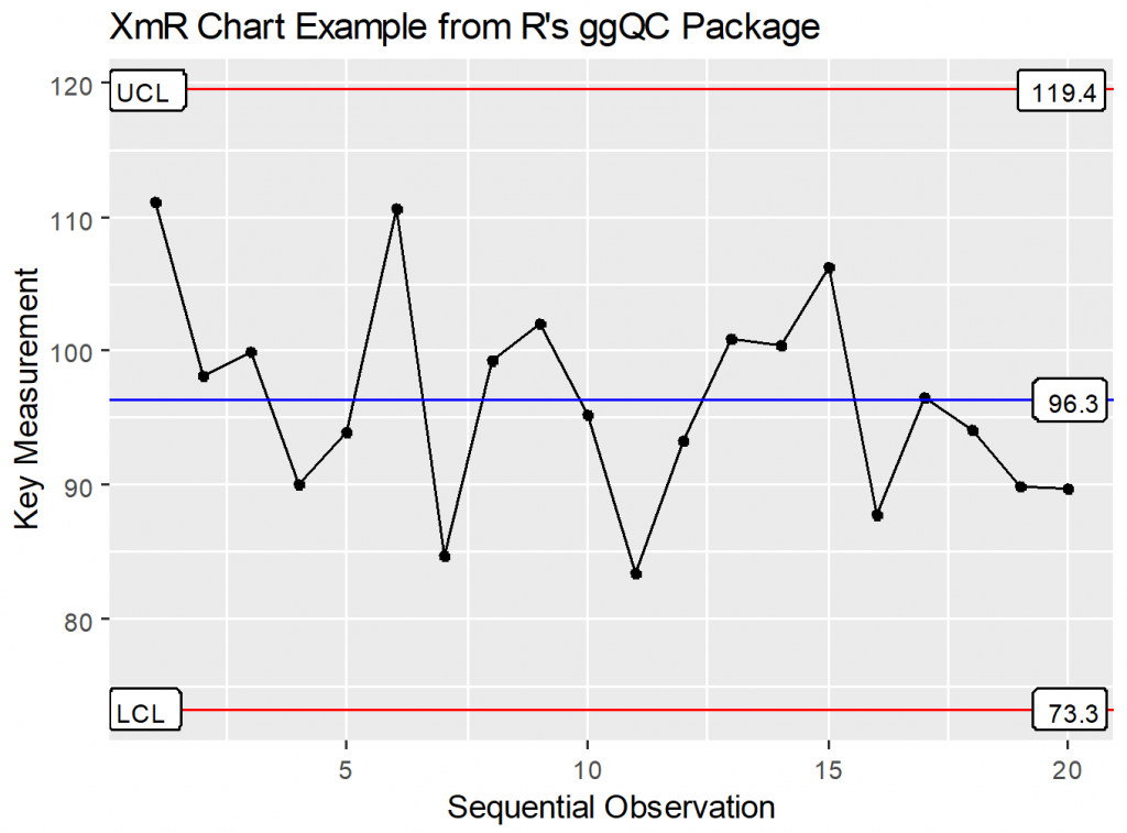
Control chart constants are the engine behind charts such as XmR, XbarR, and XbarS. And, if you’ve made a control chart by hand or sat in a class, you’ll likely have memories of bizarre constants like d2, A2, etc. To me, control chart constants are a necessary evil. Why? Because, it’s a nuisance to look up a constant to make a chart, and I suspect that has likely frightened away many would be users over the years. These days though, if you have a good piece of statistical software you won’t even see these numbers. Open source options include R’s ggQC package. An example plot is shown below. Other open source options include qcc, iqcc, and qicharts to name a few.

There are also commercially available options like minitab or JMP. Regardless of the available software, it’s still good to have a place to find these numbers when you need them and a quick explanation of their use. It’s also nice to have a sense of what these numbers physically mean.

In the next few sections, you’ll see in brief how we change quantities such as mean moving range (mR), mean range, and mean standard deviation into dispersion statistics using the control chart constants. With that dispersion statistic in hand, we can calculate control limits for our data. To begin, we’ll start with the building blocks – the bias correction factors.

Bias Correction Control Chart Constants

Bias correction constants are the fundamental quantities that allow you to calculate other higher level control constants such as A2, D3, D4, etc. Subsequent sections provide examples of how these constants are calculated.

To get a better grasp of what the bias correction factors are see my article on Estimating Control Chart Constants. There, I’ll walk you through the math and simulation to pull it all together.

Bias Correction Constants

n	d2	c4	d3	d4
2	1.1284	0.7979	0.8525	0.9539
3	1.6926	0.8862	0.8884	1.5878
4	2.0588	0.9213	0.8798	1.9783
5	2.3259	0.9400	0.8641	2.2569
6	2.5344	0.9515	0.8480	2.4717

XmR Control Chart Constants

XmR Constants

n	d2	d3	D4
2	1.1284	0.8525	3.2665

XmR Chart Calculation Reference

1.Find the center line by calculating the mean of your data points
X = mean(data)

2.Determine the mean moving range of your data points. Data must be in the sequence the samples were produced.
mR = mean(mR)

3.Convert mean(mR) to sequential deviation(Š):
Š = mR/ d2 = mR / 1.128

4.Calculate the upper and lower XmR control limits using the sequential deviation

• Lower XmR Control Limit(LCL): LCL_X = X – 3 ⋅ Š
• Upper XmR Control Limit(UCL): UCL_X = X + 3 ⋅ Š

mR Chart Calculations

Find the center line by calculating the mean moving range of your data points. Data must be in the sequence the samples were produced.
mR = mean(mR)

1.Calculate the upper and lower mR control limits

2.mR Lower Control Limit: LCL_mR = 0

3.mR Upper Control Limit: UCL_mR = 1 + 3(d3 / d2) ⋅ mR = D4 ⋅ mR

Additional XmR Constant Information

• The constant 2.66 is sometimes used to calculate XmR chart limits. The constant takes into account the 3 used to calculate the upper and lower control limit.
  2.66 = 3 / d2 = 3 / 1.12838
• Using the 2,66 constant
  Control Limits = X ± 2.66 ⋅ mR
• The D4 constant is a function of d2 and d3:
  D4 = 1 + 3(d3 / d2) = 3.2665

XbarR Control Chart Constants

XbarR charts are useful when you have sub-groups. For example:

• You have a very precise process for making cupcakes that uses a pan that can make 12 at a time. After cooking, you measure the weight of each cupcake to make sure the batter was evenly distributed. Here, the sub-group size = 12
• You have a measurement process where you make 5 measurements of a reference standard daily. Here, the subgroup size = 5

XbarR Constants

d2	d3	A2	D3	D4
1.1284	0.8525	1.8800	0.0000	3.2665
1.6926	0.8884	1.0233	0.0000	2.5746
2.0588	0.8798	0.7286	0.0000	2.2821
2.3259	0.8641	0.5768	0.0000	2.1145
2.5344	0.8480	0.4832	0.0000	2.0038

XbarR Chart Calculation Reference

1.Determine the subgroup size: n

2.Calculate the mean of each sub-group:
X = mean(each sub-group)

3.Find the center line by calculating the mean of all sub-group means:
X̿ = mean(mean(each sub-group))

4.Determine the range, Max(value)-Min(Value), for each sub-group:
R = range(each sub-group)

5.Calculate the mean range of all sub-group ranges:
R = mean(range(each sub-group))

6.Convert mean of mean ranges to within deviation, W_d:
W_d = R / d2_n

• Example 1: If n = 3 then W_d = R / 1.693
• Example 2: If n = 10 then W_d = R / 3.078

7.Determine your Upper and Lower Control Limits: Natural or Studentized

• Natural Control Limits will give you the window for the individual measurements in your process.
• • Lower XbarR Natural Control Limit: LNCL_x = X̿ – (3 ⋅ W_d) / √ 1 
  • Upper XbarR Natural Control Limit: UNCL_x = X̿ + (3 ⋅ W_d) / √ 1 

• Note: The natural limits use the √ 1  and studentized limits use √ n  (see below). It’s akin to the difference between standard deviation(SD) and standard error (SD / √ n )
• Studentized Control Limits (method 1) will give you the window for sub-group means.
• • Lower XbarR Studentized Control Limit:LCL_x = X̿ – (3 ⋅ W_d) / √ n 
  • Upper XbarR Studentized Control Limit:UCL_x = X̿ + (3 ⋅ W_d) / √ n 

• Studentized Control Limits (method 2) will give you the window for sub-group means using the control constant A2.
• A2_n = 3 / (d2_n ⋅ √ n )
• • A2_n = 3 / (d2_n ⋅ √ n )
  • Lower XbarR Studentized Control Limit: LCL_x = X̿ – R ⋅ A2_n
  • Upper XbarR Studentized Control Limit: UCL_x = X̿ + R ⋅ A2_n

Quick Demonstration: Let’s show that method 1 and 2 for calculating the control limits yields the same result.
Suppose n = 3; X̿ = 5, R = 7.
Method 1:
For n = 3, d2 = 1.6926, W_d = 7 / 1.6926 = 4.1356
LCL_x = 5 – 3 ⋅ 4.1356 / √ 3  = -2.163
UCL_x = 5 + 3 ⋅ 4.1356 / √ 3  = 12.163
Method 2:
For n = 3, A2 = 1.0233,
LCL_x = 5 – 7 ⋅ 1.0233 = -2.163
LCL_x = 5 + 7 ⋅ 1.0233 = 12.163
The Point:
For a given sub-group size = n:
A2_n = 3 / (d2_n ⋅ √ n )

R Chart Calculations

• Determine the subgroup size: n
• Calculate the range, Max(value)-Min(Value), for each sub-group:
  R = range(each sub-group)
• Determine the center line by calculating the mean range of all sub-group ranges:
  R = mean(range(each sub-group))
• Find R chart control limits:
• • R Lower Control Limit: LCL_R = D3 ⋅ R
  • R Upper Control Limit:UCL_R = D4 ⋅ R

Additional R Chart Constant Information

• The D3 constant is a function of d2, d3, and n.
  If n = 5 Then
  D3_n=5 = 1 – 3(d3_n=5 / d2_n=5) = -0.1145  →  0
• The D4 constant is a function of d2, d3, and n.
  If n = 5 Then
  D4_n=5 = 1 + 3(d3_n=5 / d2_n=5) = 2.1145

XbarS Control Chart Constants

XbarS charts come into play when you have sub-groups. For example:

• You have a very precise process for making cupcakes that uses a pan that can make 12 at a time. After cooking, you measure the weight of each cupcake to make sure the batter was evenly distributed. Here, the sub-group size = 12
• You have a measurement process where you make 5 measurements of a reference standard daily. Here, the subgroup size = 5

XbarS charts can be made with ggQC using method = “xBar.sBar”. 

XbarS Constants

n	c4	A3	B3	B4
2	0.7979	2.6587	0.0000	3.2665
3	0.8862	1.9544	0.0000	2.5682
4	0.9213	1.6281	0.0000	2.2660
5	0.9400	1.4273	0.0000	2.0890
6	0.9515	1.2871	0.0304	1.9696

XbarS Chart Calculation Reference

1.Determine the subgroup size: n

2.Calculate the mean of each sub-group: X = mean(each sub-group)

3.Find the center line by calculating the mean of all sub-group means:
X̿ = mean(mean(each sub-group))

4.Determine the standard deviation for each sub-group:
S = sd(each sub-group)

5.Calculate the mean of all sub-group standard deviations:
S = mean(sd(each sub-group))

6.Convert mean subgroup standard deviation to within deviation, W_d:
W_d = S / c4_n

• Example 1: If n = 3 then W_d = S / 0.8862
• Example 2: If n = 10 then W_d = S / 0.9727

7.Determine your Upper and Lower Control Limits: Natural or Studentized

• Natural Control Limits will give you the window for the individual measurements in your process.
• • Lower XbarS Natural Control Limit:
    LNCL_x = X̿ – (3 ⋅ W_d) / √ 1 
  • Upper XbarS Natural Control Limit:
    UNCL_x = X̿ + (3 ⋅ W_d) / √ 1 

• Note: The natural limits use the √ 1  and studentized limits use √ n  (see below). It’s akin to the difference between standard deviation(SD) and standard error (SD / √ n )
• Studentized Control Limits (method 1) will give you the window for sub-group means.
• • Lower XbarS Studentized Control Limit:
    LCL_x = X̿ – (3 ⋅ W_d) / √ n 
  • Upper XbarS Studentized Control Limit:
    UCL_x = X̿ + (3 ⋅ W_d) / √ n 

• Studentized Control Limits (method 2) will give you the window for sub-group means using the control constant A3.
• • A3_n = 3 / (c4_n ⋅ √ n )
  • Lower XbarS Studentized Control Limit:
    LCL_x = X̿ – S ⋅ A3_n
  • Upper XbarS Studentized Control Limit:
    UCL_x = X̿ + S ⋅ A3_n

Quick Demonstration: Let’s show that method 1 and 2 for calculating the control limits yields the same result.
Suppose n = 3; X̿ = 5, S = 2.
Method 1:
For n = 3, c4 = 0.8862, W_d = 2 / 0.8862 = 2.2568
LCL_x = 5 – 3 ⋅ 2.2568 / √ 3  = 1.091
UCL_x = 5 + 3 ⋅ 2.2568 / √ 3  = 8.909
Method 2:
For n = 3, A3 = 1.954,
LCL_x = 5 – 2 ⋅ 1.0233 = 1.092
LCL_x = 5 + 2 ⋅ 1.0233 = 8.908
The Point:
For a given sub-group size = n:
A3_n = 3 / (c4_n ⋅ √ n )

S Chart Calculations

1. Determine the subgroup size: n

2.Determine the standard deviation for each sub-group:
S = sd(each sub-group)

3.Calculate the mean of all sub-group standard deviations:
S = mean(sd(each sub-group))

4.Find S chart control limits:

• S Lower Control Limit:LCL_S = B3 ⋅ S
• S Upper Control Limit:UCL_S = B4 ⋅ S

Additional S Chart Constant Information

• The B3 constant is a function of c4 and n.
  If n = 5 then
  B3_n=5 = 1 – 3 / c4_n=5 ⋅ (√ 1 – (c4)² ) = -0.0889  →  0
• The B4 constant is a function of c4 and n.
  If n = 5 then
  B4_n=5 = 1 + 3 / c4_n=5 ⋅ (√ 1 – (c4)² ) = 2.0889

Summary

Tables of control chart constants and a brief explanation of how control chart constants are used in different contexts has been presented. XmR, XbarR, XbarS, mR, R, and S type control charts all require these constants to determine control limits appropriately. For XmR charts, there is only one constant needed to determine the control limits for individual observations, 1.128. However for Xbar and XbarS charts, the control constant changes as a function of sub-group size. In addition when you are calculating limits for XbarR or XbarS charts, you need to know if you are calculating natural control limits for individual measurements or studentized control limits for sub-group means. If you are doing the calculations by hand, use method 1 described above to help keep the difference between individual and studentized straight.