
- What is Data Clustering? | A Complete Guide For Beginners [ OverView ]
- What is Regression ? Know about it’s types
- What is Lasso Regression? : Learn With examples
- What is Ridge Regression? Learn with examples
- What is Linear Regression? | A Complete Guide
- What is Linear Regression in Machine Learning?
- Bagging vs Boosting in Machine Learning | Know Their Differences
- What is a Confusion Matrix in Machine Learning? : A Complete Guide For Beginners
- What Is Machine Learning | How It Works and Techniques | All you need to know [ OverView ]
- Support Vector Machine (SVM) Algorithm – Machine Learning | Everything You Need to Know
- Decision Trees in Machine Learning: A Complete Guide with Best Practices
- Pattern Recognition and Machine Learning | A Definitive Guide | Everything You Need to Know [ OverView ]
- An Overview of ML on AWS : Computer Vision, Forecasting
- Keras vs TensorFlow – What to learn and Why? : All you need to know
- Machine Learning Engineer Salary | Required Skills | Everything You Need to Know
- The Best Machine Learning Tools
- Best Deep Learning Books to Read
- Top Machine Learning Projects for Beginners
- Top Machine Learning Algorithms You Need to Know

What is Linear Regression in Machine Learning?
Last updated on 28th Jan 2023, Artciles, Blog, Machine Learning
- In this article you will get
- Introduction
- Linear regression using a simple model
- Implementation of simple linear regression algorithm using Python
- Assumptions of simple linear regression
- Conclusion
Introduction
Regression analysis may be used to make predictions about the dependent variable as a function of the independent variables.Regression models, as their name indicates, fit a line across the existing data to show the association between variables. As opposed to the straight line used in linear regression models, as is the case with logistic and nonlinear regression models, a curved line is used in the former.
Regression models may be used in a variety of contexts:
- Examination of the effects of a variable’s change on other variables.
- Future values of the dependent variable are estimated using past values of the independent variable.
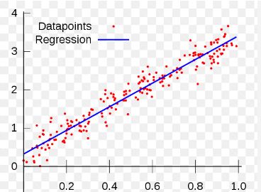
Linear regression using a simple model
The purpose of the statistical method known as simple linear regression is to establish a linear relationship between two variables. Regression estimates may have their dispersion reduced if the line’s slope and intercept are known.
The simplest form of linear regression consists of only one x-variable and one y-variable. Since the x-variable may be used apart from the predictor, it is said to be independent. y may be a dependent variable depending on your prediction objectives.
The formula for straightforward linear regression is,
- y = 0 + 1x+
- The dependent variable (y) is expected to be worth y given the value of the independent variable (x) (x).
- When x is set to 0, the expected value of y is denoted by the intercept, denoted by B0.
- The coefficient of determination, B1, indicates the expected rate of change in y given a change in x.
- The term “x” denotes the presence of a free factor ( the variable we expect is influencing y).
- If we estimate a regression coefficient, e is the error in that estimate.
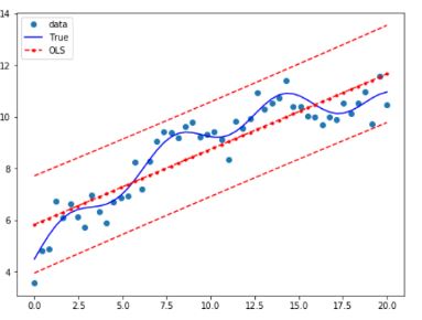
There is no guarantee that basic linear regression will help you identify a line that fits with your data, but it’s worth a go.Standard linear regression will produce an illogically sloped downward line if your data points are widely spread and have an upward trend.
Comparing the results of Simple Linear Regression with those of Multiple Linear Regression:
When attempting to anticipate the outcome of a complex process, the approach of choice is multiple linear regression rather than basic linear regression. However, when confronted with simple problems, sophisticated algorithms might be an unnecessary and even counterproductive measure.
A simple linear regression may perform an excellent job of capturing the relationship between the two variables in situations when the link between them is clear and obvious. However, you should switch from using simple regression to multiple regression when you are working with connections that are more complex.
In a multiple regression model, there is consideration given to more than one independent variable at a time. Due to the fact that it does not adhere to the same limits as the conventional regression equation, it is able to accommodate curved and non-linear relationships.
Implementation of simple linear regression algorithm using Python
- import numpy as np
- import matplotlib.pyplot as plt
- def estimate_coef(x, y):
- # number of observations/points
- n = np.size(x)
- # mean of x and y vector
- m_x = np.mean(x)
- m_y = np.mean(y)
- # calculating cross-deviation and deviation about x
- SS_xy = np.sum(y*x) – n*m_y*m_x
- SS_xx = np.sum(x*x) – n*m_x*m_x
- # calculating regression coefficients
- b_1 = SS_xy / SS_xx
- b_0 = m_y – b_1*m_x
- return (b_0, b_1)
- def plot_regression_line(x, y, b):
- # plotting the actual points as a scatter plot
- plt.scatter(x, y, color = “m”,
- marker = “o”, s = 30)
- # predicted response vector
- y_pred = b[0] + b[1]*x
- # plotting the regression line
- plt.plot(x, y_pred, color = “g”)
- # putting labels
- plt.xlabel(‘x’)
- plt.ylabel(‘y’)
- # function to show plot
- plt.show()
- def main():
- # observations / data
- x = np.array([0, 1, 2, 3, 4, 5, 6, 7, 8, 9])
- y = np.array([1, 3, 2, 5, 7, 8, 8, 9, 10, 12])
- # estimating coefficients
- b = estimate_coef(x, y)
- print(“Estimated coefficients:\nb_0 = {} \
- \nb_1 = {}”.format(b[0], b[1]))
- # plotting regression line
- plot_regression_line(x, y, b)
- if __name__ == “__main__”:
- main()
Assumptions of simple linear regression
Linearity:It is expected that x and y will have a linear link to one another. It indicates that if one value increases, the other value will also increase but at a proportionate rate. It is expected that this linearity will be seen in the scatterplot.
Independent of errors:It is of the utmost importance to check that your data is clear of any errors. If there is a relationship between the residuals and the variable, it is possible that this may cause problems with your model. Examine a scatterplot of “residuals against fits” to determine whether or not the errors are independent of one another; there should not be any indication of a correlation.
A Distribution that is normal:In addition to this, it is of the utmost importance to examine the dissemination of your data. Investigate the residuals via the lens of a histogram; it ought to be roughly normally distributed. It should also be clear from the histogram that the bulk of your observations are clustered around 0 or 1 (respectively, the highest and lowest values). It will be of assistance to you in assuring the precision and reliability of the model that you are creating.
Variance Equality:Last but not least, check to see that your data’s variances are all the same. Investigate a scatterplot for any points or locations that stand out as being significantly different from the rest of the data (you can also use statistics software like Minitab or Excel). When compared to the rest of the data, are there any points that have a big fluctuation that are considered to be outliers?
Conclusion
The use of a method known as simple linear regression may be utilised to provide an accurate prediction of a response based on the consideration of a single characteristic. It is a basic technique that may be used to the analysis of data coming from a wide range of different fields and areas of study.