Naive Bayes

What Is Naive Bayes?

Naive Bayes is among one of the simplest, but most powerful algorithms for classification based on Bayes’ Theorem with an assumption of independence among predictors. The Naive Bayes model is easy to build and particularly useful for very large data sets. There are two parts to this algorithm:

1. 1.Naive
2. 2.Bayes

The Naive Bayes classifier assumes that the presence of a feature in a class is unrelated to any other feature. Even if these features depend on each other or upon the existence of the other features, all of these properties independently contribute to the probability that a particular fruit is an apple or an orange or a banana, and that is why it is known as “Naive.”

What Is Bayes’ Theorem?

In statistics and probability theory, Bayes’ theorem describes the probability of an event, based on prior knowledge of conditions that might be related to the event. It serves as a way to figure out conditional probability.

Given a Hypothesis (H) and evidence (E), Bayes’ Theorem states that the relationship between the probability of the hypothesis before getting the evidence, P(H), and the probability of the hypothesis after getting the evidence, P(H|E),  is :

For this reason, P(H) is called the prior probability, while P(H|E) is called the posterior probability. The factor that relates the two, P(H|E)/P(E), is called the likelihood ratio. Using these terms, Bayes’ theorem can be rephrased as:

“The posterior probability equals the prior probability times the likelihood ratio.”

A little confused? Don’t worry.  Let’s continue our Naive Bayes tutorial and understand this concept with a simple concept.

Bayes’ Theorem Example

Let’s suppose we have a Deck of Cards and we wish to find out the probability of the card we picked at random to being a king, given that it is a face card. So, according to Bayes’ Theorem, we can solve this problem. First, we need to find out the probability:

• P(King) which is 4/52 as there are 4 Kings in a Deck of Cards.
• P(Face|King) is equal to 1 as all the Kings are face Cards.
• P(Face) is equal to 12/52 as there are 3 Face Cards in a Suit of 13 cards and there are 4 Suits in total.

Now, putting together all the values in the Bayes’ Equation, we get a result of 1/3.

Game Prediction Using Bayes’ Theorem

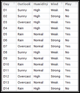
Let’s continue our Naive Bayes tutorial and predict the future with some weather data.

Here we have our data, which comprises the day, outlook, humidity, and wind conditions. The final column is ‘Play,’ i.e., can we play outside, which we have to predict.

• First, we will create a frequency table using each attribute of the dataset.

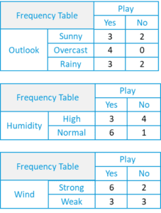
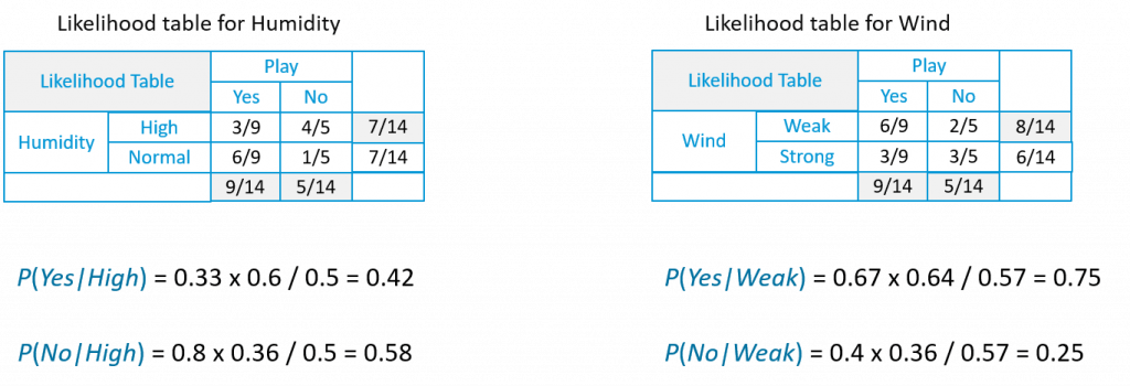
• For each frequency table, we will generate a likelihood table.

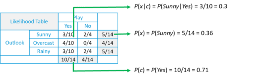
• Likelihood of ‘Yes’ given ‘Sunny‘ is:
• • P(c|x) = P(Yes|Sunny) = P(Sunny|Yes)* P(Yes) / P(Sunny) = (0.3 x 0.71) /0.36 = 0.591 
• Similarly, the likelihood of ‘No’ given ‘Sunny‘ is:
• • P(c|x) = P(No|Sunny) = P(Sunny|No)* P(No) / P(Sunny) = (0.4 x 0.36) /0.36 = 0.40
• Now, in the same way, we need to create the Likelihood Table for other attributes as well.

Suppose we have a Day with the following values :

• Outlook = Rain
• Humidity = High
• Wind = Weak
• Play = ?

So, with the data, we have to predict wheter “we can play on that day or not.”

• Likelihood of ‘Yes’ on that Day = P(Outlook = Rain|Yes)*P(Humidity= High|Yes)* P(Wind= Weak|Yes)*P(Yes)
• • = 2/9 * 3/9 * 6/9 * 9/14 = 0.0199
• Likelihood of ‘No’ on that Day = P(Outlook = Rain|No)*P(Humidity= High|No)* P(Wind= Weak|No)*P(No)
• • = 2/5 * 4/5 * 2/5 * 5/14 = 0.0166

Now, when we normalize the value, we get:

• P(Yes) =  0.0199 / (0.0199+ 0.0166) = 0.55
• P(No) = 0.0166 / (0.0199+ 0.0166)  = 0.45

Our model predicts that there is a 55% chance there will be a game tomorrow.

Naive Bayes in the Industry

Now that you have an idea of what exactly Naive Bayes is and how it works, let’s see where it is used in the industry.

RSS Feeds

Our first industrial use case is News Categorization, or we can use the term ‘text classification’ to broaden the spectrum of this algorithm. News on the web is rapidly growing where each news site has its own different layout and categorization for grouping news. Companies use a web crawler to extract useful text from HTML pages of news articles to construct a Full Text RSS. The contents of each news article is tokenized (categorized). In order to achieve better classification results, we remove the less significant words, i.e. stop, from the document. We apply the naive bayes classifier for classification of news content based on news code.

Spam Filtering

Naive Bayes classifiers are a popular statistical technique of e-mail filtering. They typically use a bag of words/features to identify spam e-mail, an approach commonly used in text classification. Naive Bayes classifiers work by correlating the use of tokens (typically words, or sometimes other things), with spam and non-spam e-mails and then, using Bayes’ theorem,  calculate a probability that an email is or is not spam.

Particular words have particular probabilities of occurring in spam emails and in legitimate emails. For instance, most email users will frequently encounter the word “Lottery” and “Luck Draw” in spam email, but will seldom see it in other emails. Each word in the email contributes to the email’s spam probability or only the most interesting words. This contribution is called the posterior probability and is computed usingBayes’ theorem. Then, the email’s spam probability is computed over all words in the email, and if the total exceeds a certain threshold (say 95%), the filter will mark the email as a spam.

Medical Diagnosis

Nowadays, modern hospitals are well equipped with monitoring and other data collection devices, resulting in enormous amount data being continuously collected through health examination and medical treatment. One of the main advantages of the Naive Bayes approach which is appealing to physicians is that “all the available information is used to explain the decision.” This explanation seems to be “natural” for medical diagnosis and prognosis, i.e. is close to the way physicians diagnose patients.

When dealing with medical data, Naive Bayes classifier takes into account evidence from many attributes to make the final prediction and provides transparent explanations of its decisions and therefore it is considered one of the most useful classifiers to support physicians’ decisions.

Weather Prediction

A Bayesian-based model for weather prediction is used, where posterior probabilities are used to calculate the likelihood of each class label for input data instance and the one with maximum likelihood is considered the resulting output.

Step-by-Step Implementation of Naive Bayes

Here we have a dataset comprising of 768 observations of women aged 21 and older. The dataset describes instantaneous measurements taken from patients, like age, blood workup, and the number of times they’ve been pregnant. Each record has a class value that indicates whether the patient suffered an onset of diabetes within 5 years. The values are 1 for Diabetic and 0 for Non-Diabetic.

Now, let’s continue our Naive Bayes tutorial and understand all the steps, one-by-one. I’ve broken the whole process down into the following steps:

• Handle data
• Summarize data
• Make predictions
• Evaluate accuracy

Step 1: Handle Data

The first thing we need to do is load our data file. The data is in CSV format without a header line or any quotes. We can open the file with the open function and read the data lines using the reader function in the CSV module.

Now we need to split the data into training and testing datasets.

Step 2: Summarize the Data

The summary of the training data collected involves the mean and the standard deviation for each attribute, by class value. These are required when making predictions to calculate the probability of specific attribute values belonging to each class value.

We can break the preparation of this summary data down into the following sub-tasks:

Separate data by class: 

Calculate mean:

Calculate standard deviation:

Summarize the dataset:

Summarize the attributes by class:

Step 3: Making Predictions

We are now ready to make predictions using the summaries prepared from our training data. Making predictions involves calculating the probability that a given data instance belongs to each class, then selecting the class with the largest probability as the prediction. We need to perform the following tasks:

Calculate the Gaussian probability density function:

Calculate class probabilities: 

Make a prediction:

Make predictions: 

Get accuracy: 

Finally, we define our main function where we call all these methods we have defined, one-by-one, to get the accuracy of the model we have created.

Output:

So here as you can see the accuracy of our model is 66%. Now, this value differs from model to model and also from the split ratio.

Now that we have seen the steps involved in the Naive Bayes Classifier, Python comes with a library, Sckit-learn, which makes all the above-mentioned steps easy to implement and use. Let’s continue our Naive Bayes tutorial and see how this can be implemented.

Naive Bayes With Sckit-learn

For our research, we are going to use the IRIS dataset, which comes with the Sckit-learn library. The dataset contains 3 classes of 50 instances each, where each class refers to a type of iris plant. Here we are going to use the GaussianNB model, which is already available in the Sckit-learn Library.

Importing Libraries and Loading Datasets

Creating Our Naive Bayes Model Using Sckit-learn

Here we have a GaussianNB() method that performs exactly the same functions as the code explained above:

Making Predictions

Getting Accuracy and Statistics

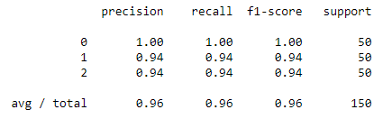
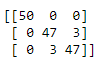
Here we will create a classification report that contains the various statistics required to judge a model. After that, we will create a confusion matrix which will give us a clear idea of the accuracy and the fitting of the model.

Classification Report:

Confusion Matrix:

Advantages

• It is not only a simple approach but also a fast and accurate method for prediction.
• Naive Bayes has very low computation cost.
• It can efficiently work on a large dataset.
• It performs well in case of discrete response variable compared to the continuous variable.
• It can be used with multiple class prediction problems.
• It also performs well in the case of text analytics problems.
• When the assumption of independence holds, a Naive Bayes classifier performs better compared to other models like logistic regression.

Disadvantages

• The assumption of independent features. In practice, it is almost impossible that model will get a set of predictors which are entirely independent.
• If there is no training tuple of a particular class, this causes zero posterior probability. In this case, the model is unable to make predictions. This problem is known as Zero Probability/Frequency Problem.

Conclusion

Congratulations, you have made it to the end of this tutorial!

In this tutorial, you learned about Naïve Bayes algorithm, it’s working, Naive Bayes assumption, issues, implementation, advantages, and disadvantages. Along the road, you have also learned model building and evaluation in scikit-learn for binary and multinomial classes.

Naive Bayes is the most straightforward and most potent algorithm. In spite of the significant advances of Machine Learning in the last couple of years, it has proved its worth. It has been successfully deployed in many applications from text analytics to recommendation engines.

I look forward to hearing any feedback or questions. You can ask your questions by leaving a comment, and I will try my best to answer it.