Simple Linear Regression | Expert’s Top Picks

• In this article you will learn:
• 1.Introduction.
• 2.Assumptions of simple linear regression.
• 3.How to perform a simple linear regression.
• 4.Simple linear regression in R.
• 5.Interpreting the results.
• 6.Presenting the results.
• 7.Conclusion.

Introduction:

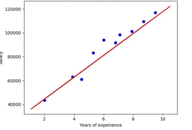
Simple linear regression is used to an estimate a relationship between the two quantitative variables.Simple linear regression are example are a social researcher interested in a relationship between income and happiness. Can survey 500 people whose incomes range from a 15k to 75k and ask them to rank their happiness on the scale from 1 to 10.Independent variable (income) and dependent variable (happiness) are the both quantitative so can do a regression analysis to see if there is linear relationship between them.If have more than a one independent variable use a multiple linear regression instead.

Assumptions of a simple linear regression:

Simple linear regression is the parametric test meaning that it makes a certain assumptions about the data. These assumptions are:

1. Homogeneity of variance (homoscedasticity): the size of an error in a r prediction doesn’t change significantly across values of the independent variable.

2. Independence of observations: an observations in the dataset were collected using a statistically valid sampling methods and there are no hidden relationships among the observations.

3. Normality: The data follows the normal distribution.

Linear regression makes the one additional assumption:

• The relationship between an independent and dependent variable is a linear: the line of best fit through a data points is a straight line.
• If data do not meet assumptions of homoscedasticity or normality may be able to use the nonparametric test instead, such as a Spearman rank test.

How to perform the simple linear regression:

Simple linear regression formula:

• y is a predicted value of a dependent variable (y) for any given value of an independent variable (x).
• B0 is a intercept the predicted value of y when a x is 0.
• B1 is a regression coefficient – how much expect y to change as a x increases.
• x is a independent variable (variable expect is an influencing y).
• e is a error of the estimate or how much variation there is in the estimate of a regression coefficient.
• Linear regression finds a line of best fit line through a data by searching for the regression coefficient (B1) that minimizes a total error (e) of the model.
• While can perform a linear regression by a hand this is a tedious process so most people use a statistical programs to help them quickly analyze a data.

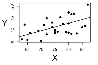
Simple linear regression in R:

• R is the free powerful and widely-used a statistical program. Download a dataset to try it and using a income and happiness example.
• Load an income.data dataset into a R environment and then run the following command to be generate a linear model describing the relationship between the income and happiness:
• R code for a simple linear regressionincome.happiness.lm <- lm(happiness ~ income, data = income.data).
• This code takes a data are have collected data = income.data and calculates an effect that the independent variable income has on dependent variable happiness using equation for a linear model: lm().

Interpreting the results:

• To view a results of model can use a summary() function in R.
• Summary(income.happiness.lm)
• This function takes a most important parameters from a linear model and puts them into the table, w
• This output table first repeats a formula that was used to create the results (‘Call’) then summarizes a model residuals (‘Residuals’) which give an idea of how well a model fits a real data.
• Next is a Coefficients’ table. The first row gives an estimates of the y-intercept and the second row gives a regression coefficient of the model.
• Row 1 ofa table is labeled (Intercept). This is y-intercept of the regression equation with the value of 0.20. can plug this into the regression equation if need to predict happiness values across a range of income that have observed.
• Next row in a ‘Coefficients’ table is income. This is a row that explains the estimated effect of an income on reported happiness.
• The Estimate column is estimated effect, also called a regression coefficient or r2 value. The number in a table (0.713) tells us that for every one unit increase in an income (where one unit of income = 10,000) there is the corresponding 0.71-unit increase in a reported happiness (where happiness is scale of 1 to 10).
• The Std. Error column displays a standard error of the estimate. This number shows how much variation there is in a estimate of the relationship between the income and happiness.
• The t value column displays a test statistic. Unless are specify otherwise the test statistic used in a linear regression is a t value from a two-sided t test. The larger a test statistic the less likely it is that are results occurred by a chance.
• The Pr(>| t |) column shows a p value. This number tells us how likely are to see the estimated effect of a income on happiness if the null hypothesis of no effect were true.
• Because p value is so low (p < 0.001), so can reject the null hypothesis and conclude that income has be statistically significant effect on happiness.
• The last three lines of a model summary are statistics about a model as a whole. The most important thing to notice here is a p value of the model. Here it is a significant (p < 0.001) which means that this model is good fit for an observed data.

Presenting the results:

When reporting the results include an estimated effect (i.e. the regression coefficient) standard error of a estimate and the p value. should also interpret the numbers to make it clear to the readers what are regression coefficient means:

• Found a significant relationship (p < 0.001) between the income and happiness (R2 = 0.71 ± 0.018), with 0.71-unit increase in a reported happiness for an every 10,000 increase in income.
• It can also be helpful to include the graph with the results. For simple linear regression and can simply plot an observations on the x and y axis and then include a regression line and regression function.

Conclusion:

Regression models explains the relationship between variables by fitting the line to the observed data. Linear regression models use a straight line while the logistic and nonlinear regression models use the curved line. Regression allows to estimate how the dependent variable changes as an independent variable(s) change.