What is Lasso Regression? : Learn With examples

• In this article you will get
• Preface to Ridge and Lasso retrogression
• Ridge Descent
• Characteristics of Ridge and Lasso retrogression
• Parameters of crest
• Ridge Retrogression( L2 Regularisation)
• Lasso Regression( L1 Regularisation)
• Limitation of Lasso Regression
• Difference between L1 and L2 Regularisation
• Advantage and Disadvantage
• Conclusion

Preface to Ridge and Lasso retrogressionn

When we point out Retrogression, we regularly point out Linear and provision Retrogression. But, that’s not the tip.I hope you discover what your particular body is pertaining to. I understood it okay and determined to explore the informed ways privately. The whole read of retreat remains identical. It means the model portions are determined to make the distinction. I explosively suggest that you simply bear a natural event numerous times before reading this. you ’ll get backing on this subject or the other item you decide on. Ridge and Lasso retrogression are important ways that generally want to produce straightforward models wherever there are a ‘ large ’ range of options.

It’s massive enough to boost the model’s tendency to overcrowding( a low of ten variables will beget overcrowding) Big enough to beget innumerous challenges. With fashionable systems, this case could arise if there are millions or lots of factors While Ridge and Lasso could appear to serve identical pretensions, the natural structures and cases of sensible use vary greatly.However, you ought to understand that they work by importing the magnitude of the portions of the options and minimizing the error between certain and factual recognition, If you ’ve detected them ahead. These are pertained to as ‘ normal ’ ways. the most distinction is still they atone for the portions.

Ridge Descent:

• Perform L2 measures, i.e. add a forfeiture up to the sq. of the scale of the portions.
• Purpose of reduction = LS Obj α *( square range of portions).

Lasso Retrogression:

• Perform L1 measure, i.e. add a penalty up to the overall volume of portions.
• Purpose of reduction = LS Obj α *( total range of portions).

Characteristics of Ridge and Lasso retrogression

• Ridge retrogression shrinks the portions and it helps to gauge back the model’s complicatedness and multicollinearity.
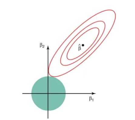
• Lasso retrogression not solely facilitates in reducingover-fitting still it’ll helpU.S. in point choice both strategies confirm portions by changing the primary purpose wherever the elliptical silhouettes hit the region of constraints. The diamond( Lasso) has corners on the axes, in discrepancy to the fragment, and whenever the elliptical region hits such a purpose, one in all the options completely vanishes.
• Cost performance of Ridge and Lasso retrogression and significance of regularization term.
• Went through some exemplifications exploiting straightforward data- sets to know retrogression toward the mean as a limiting case for each Lasso and Ridge retrogression.
• Understood why Lasso retrogression will affect point choice whereas Ridge will solely shrink portions on the point of zero.

Parameters of crest

Regularization strength; should be a positive pier. Regularization improves the literacy of the matter and reduces the friction of the estimates. Larger values specify stronger regularization. Nascence corresponds to one/( 2C) in indispensable direct models like LogisticRegression orLinearSVC.However, penalties are assumed to be specific to the targets, If an associate degree array is passed. Thus they’ve to correspond in range.

Whether to suit the intercept for thismodel.However, no intercept are utilized in computations( i, If set to false.e. X and y are anticipated to be centered).

This parameter is neglected oncefit_intercept is ready toFalse.However, the regressors X are normalized before retrogression by abating the mean and dividing by the l2- norm, If True.However, please use StandardScaler before career work on associate degree calculator with normalize = False, If you would like to standardize.

Still, X is copied; differently, it’s going to be overwritten, If True.

Maximum range of duplications for conjugate grade problem solver. For ‘sparse_cg ’ and ‘ lsqr ’ solvers, the dereliction price is decided by scipy.sparse.linalg. For ‘ slack ’ problem solvers, the dereliction price is a thousand. For ‘ lbfgs ’ problem solvers, the dereliction price is 15000.

Precision of the answer.

Solver to use within the procedure routines:

• ‘ Bus ’ chooses the problem solver mechanically supporting the kind of information.
• ‘ svd ’ uses a Singular price corruption of X to work out the Ridge portions.
• Fresh stable for singular matrices than ‘ cholesky ’.
• ‘ cholesky ’ uses the quality scipy.linalg.solve to get an unrestricted- form resolution.
• ‘sparse_cg ’ uses the conjugate grade problem solver as set up in scipy.sparse.linalg.cg. As an associate degree duplicative algorithmic rule, this problem solver is more respectable than ‘ cholesky ’ for large- scale information( possibility to line tol andmax_iter).
• ‘ lsqr ’ uses the devoted regularized least- places routine scipy.sparse.linalg.lsqr. It’s the quickest associate degreed uses a duplicative procedure.
• ‘ Slack ’ uses an arbitrary Average grade descent, and ‘ saga ’ uses its better, unprejudiced interpretation named heroic tale.
• Each way also uses an associate degree duplicative procedure, and is generally quicker than indispensable solvers once eachn_samples andn_features are giant. Note that ‘ slack ’ and ‘ saga ’ quick confluence is slightly warranted on options with around an analogous scale. you ’ll preprocess the word with a palpitation counter from sklearn.preprocessing.
• ‘ lbfgs ’ uses the L- BFGS- B algorithm rule executed in scipy.optimize.minimize. It’ll be used only if positive is True.
• All last six solvers support each thick and thin information. still, only ‘ sag ’, ‘sparse_cg ’, and ‘ lbfgs ’ support thin input oncefit_intercept is True.

Regularization ways:

There square measure basically 2 forms of regularization ways, specifically Ridge Retrogression and Lasso Regression. The manner they assign a penalty to β( portions) is what differentiates them from one another.

Ridge Retrogression( L2 Regularisation)

This fashion performs L2 regularization. The most algorithmic program behind this is frequently to change the RSS by adding the penalty that admires thesq. of the magnitude of portions. Still, it’s a way to be used once the data suffers from multiple retrogression( independent variables are extremely identified). In multiple retrogression, albeit the smallest volume places estimates( OLS) are unprejudiced, their dissonances are giant that deviates the caught on worth far from verity value. By adding a degree of bias to the retrogression estimates, crest retrogression reduces the standard crimes. It tends to resolve the multiple retrogression debit through loss parameter λ.

Lasso Regression( L1 Regularisation)

This regularization fashion performs L1 regularization. In discrepancy to Ridge Regression, it modifies the RSS by adding the penalty( loss volume) suggesting the addition of the price of portions. Looking at the equation below, we’re able to observe that just like Ridge Regression, Lasso( Least Absolute Shrinkage and Choice Operator) jointly penalizes absolutely the size of the retrogression portions. In addition to the present, it’s quite able to reduce the variability and raise the delicacy of statistical retrogression models.

Limitation of Lasso Regression

Still, Lasso can decide at most n predictors asnon-zero, although all predictors are unit applicable( or are also employed in the check set), If the volume of predictors( p) is larger than the volume of compliances( n). In similar cases, Lasso generally must struggle with similar kinds of information.However, also LASSO retrogression chooses one in every of them every{ which way} which is n’t smart for the interpretation of knowledge, If there are unit 2 or fresh extremely direct variables. Lasso retrogression differs from crest retrogression in that it uses absolute values among the penalty performed, rather than that of places. This ends up in penalizing( or equally constrictive the addition of absolutely the values of the estimates) values that causes a number of the parameter estimates to show out specifically zero. The fresh penalty is applied, the freshest the estimates get shrunken towards temperature.

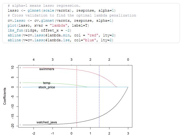
Syntax with exemplifications:

• An illustration of Ridge retreat.
• At this stage, we frequently stop and go live to show how to apply the Ridge Retrogression rule.
• First, let’s introduce a set of custom reclamation data.
• The casing database may be a typical machine learning database conforming to 506 lines of information with thirteen input variations and target numerical variations.
• Using a 10-fold double- factor-positive cross-check check harness, the unit of total perceptivity is ready to make a total error( MAE) for a reference of0.5 adozen.6.
• The database includes prognosticating the value of the home given the details of the casing community within the yankee city of Boston.

5 rows x fourteen columns

Ironically, the word lambda is arranged with the argument “ nascence ” and the system used in the section. The dereliction price is1.0 or full forfeiture.

Frame model:

We can test the Ridge Retrogression model on the casing database continuously to confirm 10 times and report a common mean absolute( MAE) error on the database.For illustration it examines the Ridge Retrogression system in the casing database and reports a standard MAE for all 3 duplicates of 10 times the contrary assurance.Your specific issues may vary depending on the arbitrary nature of the tutoring law.

In this case, we tend to stand still and be prepared to see that the model has achieved MAE in terms of tripartite.382. Means MAE three.382(0.519).We may try to use Ridge Regression as our final model and make prognostications on new information. This can be achieved by modeling all available information and active vaticination() function, across the entire information line.

How its workshop?

The L1 performance provides affair in double weights from 0 to 1 in model features and was espoused to reduce the number of features in a large size database. The drop in Lasso is analogous to the decline of the line, but uses a process “ drop ” in which the cut- off portions drop towards zero. Lower lariat allows you to reduce or make these portions equal to avoid overcrowding and make them work more on different databases.

Ridge Retrogression is a system of analyzing multiple retrospective data that suffers from multicollinearity. By adding a certain degree of bias to the retrogression conditions, the crest retreat reduces common crimes. It’s hoped that the result will be to give more accurate measures.

Why is it important?

In short, crest and lariat retreat are advanced retraction styles to prognosticate, rather than enterprise.Normal reversal gives you a neutral divagation measure( large probability values ” as noted in the data set ”).Ridge and lasso campo allow you to typically make portions( “ loss ”). This means that the estimated portions are pushed to 0, making them work more on new data sets( “ prophetic prognostications ”).

In both the crest and the lariat you have to set what’s called a “ meta parameter ” which describes how the aggressive adaptation is performed. Meta parameters are generally named with the contrary evidence. For Ridge reclamation the meta parameter is generally called “ nascence ” or “ L2 ”; it simply describes the power of adoption. In LASSO the meta parameter is generally called ” lambda ”, or ” L1 ”. In discrepancy to Ridge, the LASSO familiarity will actually set the less important prognostications to 0 and help you in choosing prognostications that can be left out of the model. These two styles are integrated into the ” Elastic Net ” Regularisation.

Then, both parameters can be set, with “ L2 ” defining customization power and “ L1 ” and the minimum of the asked results. Indeed though the line model may be applicable to the data handed for modeling, it isn’t really guaranteed to be the stylish predictable data model.Still, and the model we use is too complex to perform the task, what we actually do is put a lot of weight on any possible changes or variations of the data, If our introductory data follows a fairly simple model. Our model is extremely responsive and compensates for indeed the fewest change in our data. People in the field of calculi and machine literacy call this situation overfitting.However, it turns out that direct models may be overcrowded, If you have features in your database that are nearly linked in line with other features.Ridge Regression, avoids imbrication by adding forfeitures to models with veritably large portions.

Difference between L1 and L2 Regularisation

The main difference between these styles is that the Lasso reduces the unnecessary element to zero therefore, barring a specific point fully. Thus, this works best for point selection when we’ve a large number of features. Common styles similar as rear verification, retrospective follow- up runningover-install and point point selection work well with a small set of features but these ways are a good option.

Advantage and Disadvantage

Advantage:

• It avoids overfilling the model.
• They don’t bear fair measures.
• They can add enough bias to make measures a fairly dependable estimate of real mortal figures.
• They still work well in large multivariate data cases with a number of prognostications§ larger than the reference number( n).
• The crest scale is excellent for perfecting the rate of small places when there’s multicollinearity.

Disadvantage:

• They include all the prognostications in the final model.
• Can’t select features.
• They shrink the measure to zero.
• They trade the difference for bias.

Conclusion

Now that we’ve a good idea of how the crest and lariat retrogression work, let’s combine our understanding by comparing it and try to appreciate their specific operating conditions. I’ll also compare them with other styles. Let’s assay these under three pails.