Ridge and Lasso Regression (L1 and L2 regularization) Explained Using Python – Expert’s Top Picks

• In this article you will get
• 1.Introduction to Ridge and lasso regression
• 2.Characteristics of Ridge and lasso regression
• 3.Parameters of ridge
• 4.Regularization techniques
• 5.How its works?
• 6.Why is it important?
• 7.Difference between L1 and L2 Regularisation
• 8.Advantage and Disadvantage
• 9.Conclusion

Introduction to Ridge and lasso regression

When we signify Regression, we tend to often signify Linear and provision Regression. But, that’s not the tip. one-dimensionality and order are the foremost modern members of the retreat family. Last week, I saw a recorded speech at the NYC Information Science Academy from Owen Zhang, Chief Product Officer at DataRobot. He said, ‘if you utilize reciprocity, you need to be really special!’. I hope you discover what your personal body is touching on. I understood it okay and determined to explore the acquainted with techniques intimately. During this article, I even diagrammatic the difficult science behind ‘Ridge Regression’ and ‘Lasso Regression’ that are at the foremost common ways that are utilized in information science, sadly still not used by many.

The whole scan of retreat remains identical. It suggests that the model coefficients are determined to create excellence. I powerfully counsel merely|that you just} simply bear a happening over and over before reading this. you’ll get help on this subject or the opposite item you opt on. Ridge and Lasso regression are powerful techniques that generally need to supply easy models where there are a ‘large’ variety of choices. Here the word ‘big’ can mean any of two things:

It is huge enough to spice up the model’s 10dency to overcrowding (a low of ten variables can cause overcrowding) sufficiently big to cause uncounted challenges. With modern systems, this case might arise if there are millions or scores of factors whereas Ridge and Lasso might seem to serve identical goals, the natural structures and cases of wise use vary greatly. If you’ve detected them before, you need to perceive that they work by considering the magnitude of the coefficients of the choices and minimizing the error between bound and actual recognition. These are observed as ‘normal’ techniques. the foremost distinction is but they compensate for the coefficients:

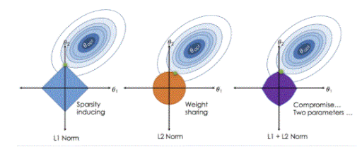
Ridge Descent:

Perform L2 measurements,i.e. add a fine up to the sq. of the dimensions of the coefficients.

Lasso Regression:

Perform L1 live, i.e. add a penalty up to the general amount of coefficients.

Characteristics of Ridge and lasso regression

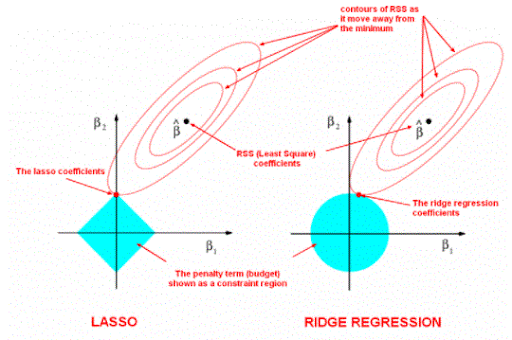
Ridge regression shrinks the coefficients and it helps to cut back the model quality and multiple regression. Lasso regression not alone facilitates in reducing over-fitting but it’ll facilitate U.S. in feature alternatives each way to ensure coefficients by finding the first purpose where the elliptical contours hit the region of constraints. The diamond (Lasso) has corners on the axes, in distinction to the disk, and whenever the elliptical region hits such a purpose, one altogether the choices absolutely vanishes.

Went through some examples exploiting easy data-sets to grasp regression toward the mean as a limiting case for every Lasso and Ridge regression.

Understood why Lasso regression can lead to feature alternatives whereas Ridge can alone shrink coefficients on the brink of zero.

Parameters of ridge

Regularization strength; ought to be a positive float. Regularization improves the training of the matter and reduces the variance of the estimates. Larger values specify stronger regularization. Alpha corresponds to at least one / (2C) in different linear models like LogisticRegression or LinearSVC. If an associate degree array is passed, penalties are assumed to be specific to the targets. thus they need to correspond in varying ways.

Whether to suit the intercept for this model. If set to false, no intercept ar used in calculations.

This parameter is neglected once fit_intercept is prepared to False. If True, the regressors X are normalized before regression by subtracting the mean and dividing by the l2-norm. If you’d wish to standardize, please use StandardScaler before career work on a degree calculator with normalize=False.

If True, X are copied; else, it’s getting to be overwritten.

Maximum variety of iterations for conjugate gradient thinker. For ‘sparse_cg’ and ‘lsqr’ solvers, the default value is set by scipy.sparse.linalg. For ‘sag’ downside solvers, the default value could be a thousand. For ‘lbfgs’ downside solvers, the default value is 15000.

Precision of the solution.

Solver to use at intervals the procedure routines:

‘auto’ chooses the matter thinker automatically supporting the sort of knowledge.

‘svd’ uses a Singular value Decomposition of X to figure out the Ridge coefficients. Further stable for singular matrices than ‘cholesky’.

‘cholesky’ uses the standard scipy.linalg.solve to induce a closed-form resolution.

‘sparse_cg’ uses the conjugate gradient thinker as found in scipy.sparse.linalg.cg. As an associate degree repetitious formula, this thinker is further acceptable than ‘cholesky’ for large-scale info (possibility to line tol and max_iter).

‘lsqr’ uses the dedicated regular least-squares routine scipy.sparse.linalg.lsqr. It’s the fastest associate degreed using an associate repetitious procedure.

‘sag’ uses a random Average Gradient descent, and ‘saga’ uses its improved, unbiased version named adventure story. Every approach to boot uses an associate degree repetitious procedure, and is typically faster than different solvers once every n_samples and n_features are large. Note that ‘sag’ and ‘saga’ fast convergence is barely guaranteed on choices with around the same scale.

You’ll preprocess the information with a counter from sklearn.preprocessing.

‘lbfgs’ uses the L-BFGS-B formula implemented in scipy.optimize.minimize. it’ll be used on condition that positive is True.

All last six solvers support every dense and skinny info. However, only ‘sag’, ‘sparse_cg’, and ‘lbfgs’ support skinny input once fit_intercept is True.

Regularization techniques

There unit of measurement in the main a pair of varieties of regularization techniques, specifically Ridge Regression and Lasso Regression.

Lasso Regression (L1 Regularisation):

This regularization technique performs L1 regularization. In distinction to Ridge Regression, it modifies the RSS by adding the penalty (shrinkage quantity) resembling the addition of the value of coefficients. gazing the equation below, we tend to square measure ready to observe that rather like Ridge Regression, Lasso (Least Absolute Shrinkage and selection Operator) put together penalizes fully the scale of the regression coefficients. additionally to this, it’s quite capable of reducing the variability and raising the accuracy of statistical method models.

Limitation of Lasso Regression:

If the amount of predictors (p) is larger than the amount of observations (n), Lasso will decide at most n predictors as non-zero, though all predictors square measure unit relevant (or also are used within the check set). In such cases, Lasso usually should struggle with such types of data. If their square measure unit a pair of or extra very linear variables, then LASSO regression chooses one in each of them that isn’t good for the interpretation of information. Lasso regression differs from ridge regression; therein it uses absolute values among the penalty performed, rather than that of squares. This finishes up in penalizing (or equivalently constrictive the addition of fully the values of the estimates) values that causes a variety of the parameter estimates to point out specifically zero. The extra penalty is applied, the extra the estimates get shrunken towards temperature. This helps to variable alternatives out of a given vary of n variables.

Syntax with examples:

An example of Ridge retreat:

At this stage, we regularly stop and go live to point out the way to apply the Ridge Regression rule.

First, let’s introduce a group of custom retrieval information. We tend to tend to square live to use the housing information.

The housing information is also a typical machine learning information consisting of 506 lines of knowledge with 13 input variations and target numerical variations.

Using a 10-fold double-factor-positive control check harness, the unit of total sensitivity is prepared to create a complete error (MAE) for a reference of zero.5 adozen.6. The foremost economical model unit of measurement is prepared to perform MAE within the same check instrument with relevancy one.9. This provides the performance parameters for this information.

The information includes predicting the worth of the house given the small print of the housing community at intervals the american city of Beantown.

• Housing information Set (housing.csv).
• Housing Description (housing.names).
• You do not have to be forced to maneuver a database; we regularly stop live to mechanically transmit it as a part of our processed models.

The example below is downloaded with a great deal of informations like Pandas DataFrame and summarizes the sort of database and compiles the primary five lines of knowledge.

Establishing a model validates 506 data lines and 13 input variables furthermore as one target numerical variable (14 in total). sq. mensuration adjusted} in addition see that each variable input unit of variety|variety} could be a number.

We can check the Ridge Regression model on the housing information incessantly to substantiate ten times and report a typical mean absolute (MAE) error on the information.

For example it examines the Ridge Regression system within the housing information and reports a regular MAE for all three duplicates of ten times the alternative assurance.

Your specific outcomes could vary looking at the random nature of the teaching law. contemplate running an occurrence over and another time.

In this case, we tend to square still and be ready to ascertain that the model has achieved MAE in terms of threefold.382.

Means MAE: 3.382 (0.519)

We could attempt to use Ridge Regression as our final model and build predictions on new data.

This can be achieved by modeling all offered data and active prediction () performance, across the complete data line.

How its works?

The L1 performance provides output in binary weights from zero to one in model options and was adopted to cut back the amount of options in a very massive size information. The L2 suspension spreads error targets across all weights resulting in a lot of correct customizable final models.

The decrease in Lasso is comparable to the decline of the road, however it uses a method “decrease” within which the cut-off coefficients decrease towards zero. Lower lasso permits you to cut back or build these coefficients adequately to avoid overcrowding and build them work higher on completely different databases.

Ridge Regression could be a technique of analyzing multiple retrospective information that suffers from multiple regression. By adding an exact degree of bias to the regression ratings, the ridge retreat reduces common errors. It’s hoped that the results are going to be to produce a lot of correct measurements.

Why is it important?

In short, ridge and lasso retreat square measure advanced retraction strategies to predict, instead of speculation. Normal reversal provides you a neutral deviation constant (large chance values ​​”as noted within the knowledge set”).

Ridge and lasso downs enable you to usually create coefficients (“shrinkage”). This suggests that the calculable coefficients square measure pushed to zero, creating them work higher on new knowledge sets (“predictive predictions”). This permits you to use advanced models and avoid over-installation at identical times.

In each ridge and therefore the lasso you’ve got to line what’s known as a “meta parameter” that describes however the aggressive adjustment is performed. Meta parameters square measure sometimes hand-picked with the other confirmation. For Ridge retrieval the meta parameter is typically known as “alpha” or “L2”; it merely describes the ability of adaptation. In LASSO the meta parameter is typically known as “lambda”, or “L1”. In distinction to Ridge, the LASSO familiarity can truly set the less significant predictions to zero and assist you in selecting predictions that may be unseen from the model. These 2 strategies square measure integrated into the “Elastic Net” Regularisation.

Here, each parameter is set, with “L2” process customization power and “L1” and therefore the minimum of the specified results. Even though the road model could also be relevant to the info provided for modeling, it’s not extremely certain to be the most effective foreseeable knowledge model.

If our basic knowledge follows a comparatively straightforward model, and therefore the model we have a tendency to use is just too advanced to perform the task, what we have a tendency to truly do is place tons of weight on any attainable changes or variations of the info. Our model is extraordinarily responsive and compensates for even the slightest amendment in our knowledge. folks within the field of math and machine learning decide this example is overfitting. If you’ve got options in your info that square measure closely coupled in line with alternative options, it seems that linear models could also be overcrowded. Ridge Regression, avoids overlap by adding fines to models with terribly giant coefficients.

Difference between L1 and L2 Regularisation

The main distinction between these strategies is that the Lasso reduces the non-essential component to zero, eliminating a selected feature utterly. Therefore, this works best for feature choice after we have an oversized variety of options. Common strategies like reverse verification, retrospective follow-up handling over-install and feature choice work well with a tiny low set of options however these techniques square measure a decent possibility once addressing an oversized set of options.

Advantage and Disadvantage

• It avoids overloading the model.
• They do not need honest measurements.
• They can add enough bias to form measurements and a reasonably reliable estimate of real human numbers.
• They still work well in giant variable knowledge cases with {a variety|variety} of predictions & larger than the reference number (n).
• The ridge scale is great for up the magnitude relation of little squares once there’s multiple regression.
• They embrace all the predictions within the final model.
• Can’t choose options.
• They shrink the constant to zero.
• They trade the distinction for bias.

Conclusion

Now that we’ve a decent plan of how the ridge and lasso regression work, let’s try and mix our understanding by scrutinizing it and checking out to understand their specific operation conditions. I will be able to additionally compare them with alternative strategies. Let’s analyze these below 3 buckets:

1. Vital variations:

Ridge: Includes all (or no) options within the model. Therefore, the most advantage of ridge retraction is the reduction of the constant and therefore the reduction of the quality of the model.

Lasso: With slower coefficients, lasso makes feature choice moreover. (Remember the ‘selection’ fully lasso form?) As we’ve seen before, some coefficients become precisely zero, the equivalent of an exact component extracted from the model.

2. Commonplace conditions of use:

Ridge: Used extensively to stop overcrowding. because it incorporates all the options, it’s not terribly helpful within the case of #supported options, if they mean millions, because it can gift machine challenges.

Lasso: because it offers a number of solutions, it’s sometimes Associate in Nursing elective model (or various to the present concept) in modeling things wherever the #million options or additional. In such a case, finding a tiny low answer is a nice calculation as options with zero coefficients will merely be unnoted.

It is not troublesome to visualize why the strategies that follow the steps become thus troublesome to use in things of high magnitude. Thus, lasso offers nice advantages.

3. Presence of extremely connected options:

Ridge: it always works well even once there square measures extremely connected options because it can integrate all of them into the model, however the coefficients are distributed between them, depending on the relative.

Lasso: Ignorantly selects any feature among the foremost connected and lowers the coefficients otherwise to zero. Also, the chosen variables change haphazardly by dynamically the parameters of the model. This sometimes doesn’t work o.k. compared to ridge receding.

This lasso arrangement is seen within the example we have a tendency to mention higher than. As we have a tendency to apply polynomial regression, the variables were extremely related to. (Not positive why? investigate the info.corr () output. Therefore, we have a tendency to discovered that even the littlest alpha values provided a big minimum (i.e. the very best coefficients square measure # like zero).