What is Normality Test in Minitab?

The one-sample t-test is used to determine whether a sample comes from a population with a specific mean. This population mean is not always known, but is sometimes hypothesized.

For example, imagine that an academic was conducting research on the relationship between exam performance and revision time, but wanted to first check whether his 100 participants reflected the national average in terms of their academic ability, measured in terms of their GMAT score. The academic could use a one-sample t-test to compare the GMAT score of the 100 participants against the national average. Alternately, imagine that a lecturer believed her course required 10 hours of study time per week and wanted to determine whether students spent this amount of time studying. The lecturer could use a one-sample t-test to compare the weekly study time of a sample of 20 students to the suggested 10 hours.

In this guide, we show you how to carry out a one-sample t-test using Minitab, as well as interpret and report the results from this test. However, before we introduce you to this procedure, you need to understand the different assumptions that your data must meet in order for a one-sample t-test to give you a valid result. We discuss these assumptions next.

Perform a normality test

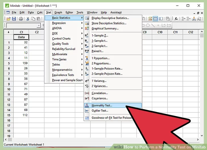
Choose Stat > Basic Statistics > Normality Test. The test results indicate whether you should reject or fail to reject the null hypothesis that the data come from a normally distributed population. You can do a normality test and produce a normal probability plot in the same analysis. The normality test and probability plot are usually the best tools for judging normality.

Types of normality tests

The following are types of normality tests that you can use to assess normality.

Anderson-Darling test :

This test compares the ECDF (empirical cumulative distribution function) of your sample data with the distribution expected if the data were normal. If the observed difference is adequately large, you will reject the null hypothesis of population normality.

Ryan-Joiner normality test :

This test assesses normality by calculating the correlation between your data and the normal scores of your data. If the correlation coefficient is near 1, the population is likely to be normal. The Ryan-Joiner statistic assesses the strength of this correlation; if it is less than the appropriate critical value, you will reject the null hypothesis of population normality. This test is similar to the Shapiro-Wilk normality test.

Kolmogorov-Smirnov normality test :

This test compares the ECDF (empirical cumulative distribution function) of your sample data with the distribution expected if the data were normal. If this observed difference is adequately large, the test will reject the null hypothesis of population normality. If the p-value of this test is less than your chosen α, you can reject your null hypothesis and conclude that the population is non-normal.

Comparison of Anderson-Darling, Kolmogorov-Smirnov, and Ryan-Joiner normality tests :

Anderson-Darling and Kolmogorov-Smirnov tests are based on the empirical distribution function. Ryan-Joiner (similar to Shapiro-Wilk) is based on regression and correlation.

All three tests tend to work well in identifying a distribution as not normal when the distribution is skewed. All three tests are less distinguishing when the underlying distribution is a t-distribution and nonnormality is due to kurtosis. Usually, between the tests based on the empirical distribution function, Anderson-Darling tends to be more effective in detecting departures in the tails of the distribution. Usually, if departure from normality at the tails is the major problem, many statisticians would use Anderson-Darling as the first choice

The one-sample t-test is used to determine whether a sample comes from a population with a specific mean. This population mean is not always known, but is sometimes hypothesized.

For example, imagine that an academic was conducting research on the relationship between exam performance and revision time, but wanted to first check whether his 100 participants reflected the national average in terms of their academic ability, measured in terms of their GMAT score. The academic could use a one-sample t-test to compare the GMAT score of the 100 participants against the national average. Alternately, imagine that a lecturer believed her course required 10 hours of study time per week and wanted to determine whether students spent this amount of time studying. The lecturer could use a one-sample t-test to compare the weekly study time of a sample of 20 students to the suggested 10 hours.

Minitab

Assumptions

A one-sample t-test has four assumptions. You cannot test the first two of these assumptions with Minitab because they relate to your study design and choice of variables. However, you should check whether your study meets these two assumptions before moving on. If these assumptions are not met, there is likely to be a different statistical test that you can use instead. Assumptions #1 and #2 are explained below:

• Assumption 1: Your dependent variable should be measured at a continuous level (i.e., it is an interval or ratio variable). Examples of continuous variables include height (measured in feet and inches), temperature (measured in °C), salary (measured in US dollars), revision time (measured in hours), intelligence (measured using IQ score), firm size (measured in terms of the number of employees), age (measured in years), reaction time (measured in milliseconds), grip strength (measured in kg), power output (measured in watts), test performance (measured from 0 to 100), sales (measured in number of transactions per month), academic achievement (measured in terms of GMAT score), and so forth. If you are unsure whether your dependent variable is continuous (i.e., measured at the interval or ratio level), see our Types of Variable guide.
• Assumption 2: The data are independent (i.e., not correlated/related), which means that there is no relationship between the observations. This is more of a study design issue than something you can test for, but it is an important assumption of the one-sample t-test.

Assumptions 3 and 4 relate to the nature of your data and can be checked using Minitab. You have to check that your data meets these assumptions because if it does not, the results you get when running a one-sample t-test might not be valid. In fact, do not be surprised if your data violates one or more of these assumptions. This is not uncommon. However, there are possible solutions to correct such violations (e.g., transforming your data) such that you can still use a one-sample t-test. Assumptions #3 and #4 are explained below:

• Assumption 3: There should be no significant outliers. An outlier is simply a case within your data set that does not follow the usual pattern. For example, consider a study examining the test anxiety of 500 students where anxiety was measured on a scale of 0-100, with 0 = no anxiety and 100 = maximum anxiety. The mean test anxiety score was 56 and the vast majority of students scored between 42 and 70. However, one student scores just 2 on the scale, with the second lowest test anxiety score being 36. As such, a student scoring just 2 on the scale “could” be considered an outlier. Where a score is an outlier this is problematic because outliers can have a disproportionately negative effect on the one-sample t-test, reducing the accuracy of its results. Fortunately, when using Minitab to run a one-sample t-test on your data, you can easily detect possible outliers.
• Assumption 4: Your dependent variable should be approximately normally distributed. We talk about the one-sample t-test only requiring approximately normal data because it is quite “robust” to violations of normality, meaning that the assumption can be a little violated and still provide valid results. You can test for normality using the Shapiro-Wilk test of normality, which is easily tested for using Minitab.

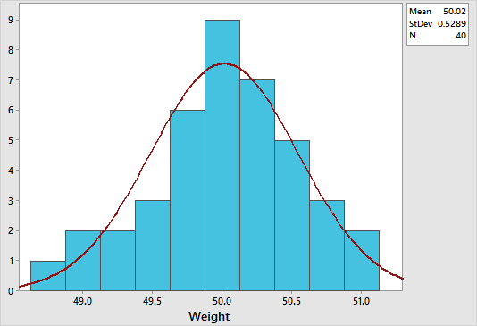
Histograms:

Histograms are efficient graphical methods for describing the distribution of data. It is always a good practice to plot your data in a histogram after collecting the data. This will give you an insight about the shape of the distribution and whether it is normal or not. If the data is symmetrically distributed and most results are located in the middle, we can say that the data is normally distributed.

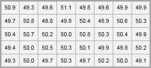
Suppose that a line manager is seeking to assess how consistently a production line is producing. He is interested in the weight of a food products with a target of 50 grams per item. He takes a random sample of 40 products and measures their weights. For this example, we may use the product_weight worksheet. Remember to copy the data from the Excel worksheet and paste it into the Minitab worksheet.

To create a histogram in Minitab, select Graph > Histogram > With Fit, specify the column of data to analyze, in this case ‘product weight’, and then click OK. The figure below shows a histogram which suggests that the data is normally distribution. Notice how the data is symmetrically distributed and concentrated in the center of the histogram.

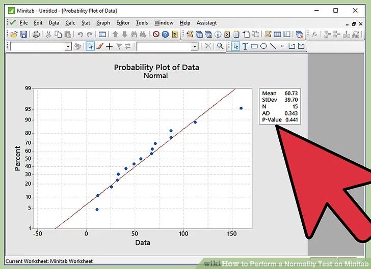
Normal Probability Plots:

We can also construct a Normal Probability Plot to test the assumption of normality. This provides a more decisive approach for deciding if a data set is normally distributed. All points for a normal distribution should approximately form a straight line that falls between 95% confidence interval limits.

To create a normal probability plot in Minitab, select Graph > Probability Plot > Single, specify the column of data to analyze, leave the distribution option to be normal, and then click OK. Here is a screenshot of the example result for our previous product_weight example:

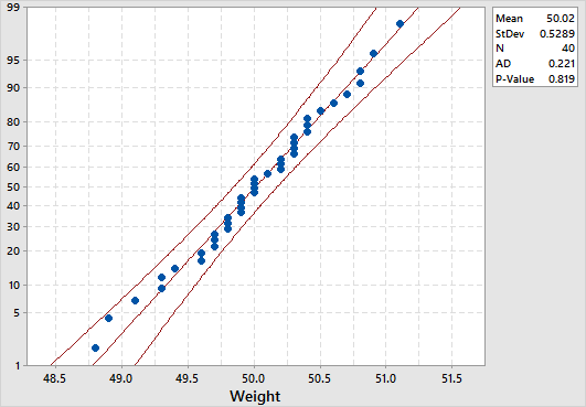
The normal distribution is a good fit if the data points approximately follow a straight line. In our example, the data points approximately follow a straight line that falls mainly between the 95% confidence interval limits, and so it can be concluded that the data is normally distributed.

Anderson-Darling Normality Test:

The Anderson-Darling Normality Test measures how well the data follow the normal distribution (or any particular distribution). It is a statistical test that compares the actual distribution with the theoretical normal distribution. A lower p-value than the significance level (normally 0.05) indicates a lack of normality in the data (regardless of the AD value). Remember to keep your eyes on the histogram and the normal probability plot in conjunction with the Anderson-Darling test before making any decision.

To conduct an Anderson-Darling normality test in Minitab, select Stat > Basic Statistics > Normality Test, specify the column of data to analyze, then specify the test method to be Anderson-Darling, and then click OK. The p-value in our product_weight example is 0.819 which suggests that the data follow the normal distribution. Note that both the graphical summary and the probability plot displays Anderson-Darling normality test results by default.

How to Perform a Normality Test on Minitab

Before you start performing any statistical analysis on the given data, it is important to identify if the data follows normal distribution. If the given data follows normal distribution, you can make use of parametric tests (test of means) for further levels of statistical analysis. If the given data does not follow normal distribution, you would then need to make use of non-parametric tests (test of medians). As we all know, parametric tests are more powerful than nonparametric tests. Hence, checking the normality of the given data becomes all the more important.

Steps

1. Write the hypothesis. A good way to perform any statistical analysis is to begin by writing the hypothesis. For normality test, the null hypothesis is “Data follows a normal distribution” and alternate hypothesis is “Data does not follow a normal distribution”.

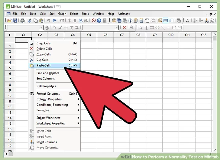
2. Choose the data. Select and copy the data from the spreadsheet on which you want to perform the normality test.

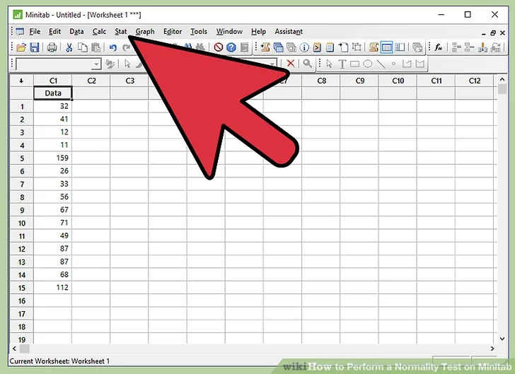
3. Paste the data in Minitab worksheet. Open Minitab and paste the data in Minitab worksheet.

4. Click “Stat”. In the menu bar of Minitab, click on Stat.

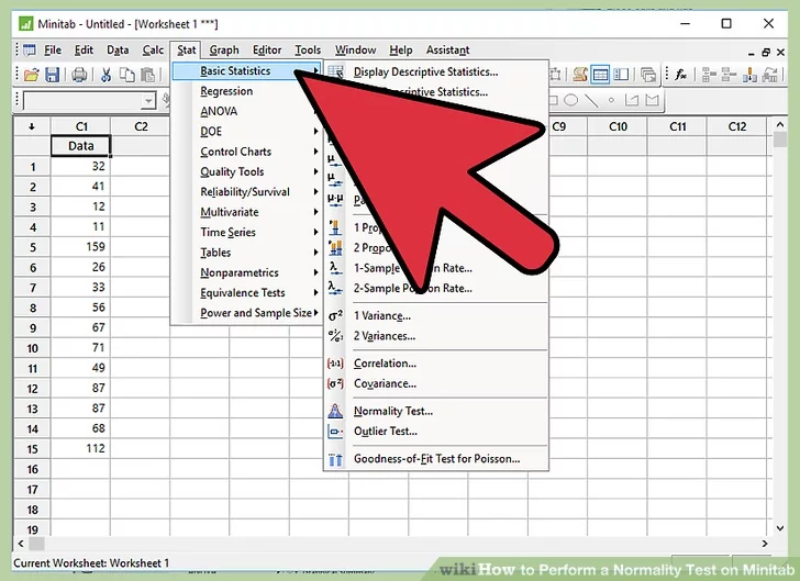
5. Click “Basic Statistics”.

6. Click “Normality Test”

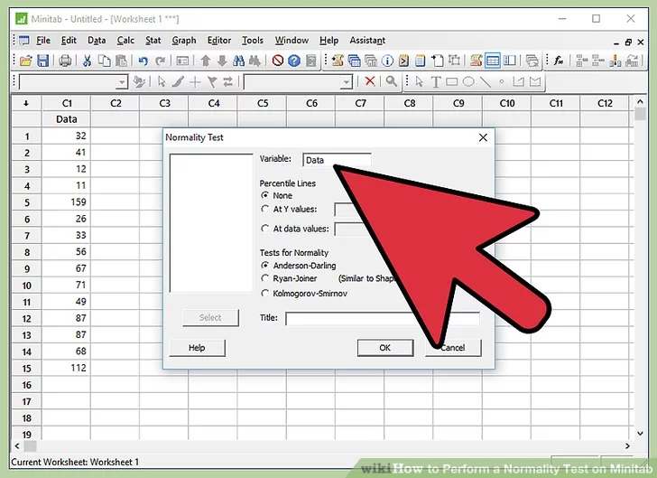
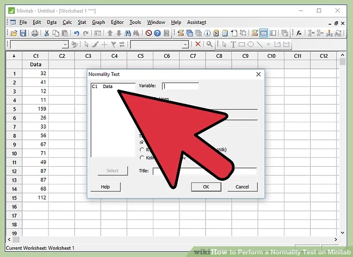
7. Select data. A small window named “Normality Test” will pop-up on the screen. Click on the available option inside the white box and then Click “Select”.

• Be aware that the “Variable” tab will have the name of selected data.

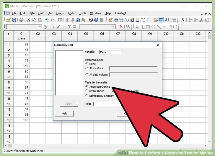
• Also be aware that “Anderson-Darling” is already selected under “Tests for Normality”. Anderson-Darling is the most widely used Normality test. Hence, in Minitab, the default selection of Tests for Normality is “Anderson-Darling”.

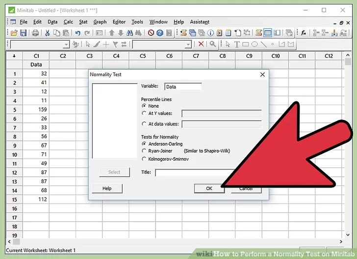
8. Click “Ok”.

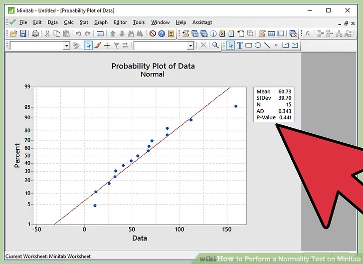
9. Understand the p-value displayed in the Normal Probability Plot. A normal probability plot will appear on the screen.

• Please observe if the p-value displayed in the normal probability plot is greater than 0.05 or is it lesser than 0.05.

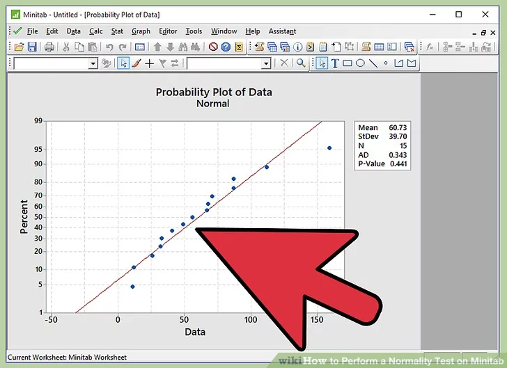
10.Infer the results. As described in the step of writing the hypothesis, if we fail to reject the null hypothesis, the inference will be “Data follows a normal distribution”. If we reject the null hypothesis, the inference will be “Data does not follow a normal distribution”. Let’s link the p-value to the written hypothesis.

11. Do not reject null hypothesis if p-value is greater than 0.05. If the p-value observed in normal probability plot is greater than 0.05, we fail to reject the null hypothesis. Thus the inference is “Data follows a normal distribution”.

12. Reject the null hypothesis if p-value is lesser than 0.05. If the p-value observed in normal probability plot is less than 0.05, we reject the null hypothesis. Thus the inference is “Data does not follow a normal distribution”.