Machine Learning-Random Forest Algorithm Tutorial

Random Forest is a popular machine learning algorithm that belongs to the supervised learning technique. It can be used for both Classification and Regression problems in ML. It is based on the concept of ensemble learning, which is a process of combining multiple classifiers to solve a complex problem and to improve the performance of the model.

As the name suggests, “Random Forest is a classifier that contains a number of decision trees on various subsets of the given dataset and takes the average to improve the predictive accuracy of that dataset.” Instead of relying on one decision tree, the random forest takes the prediction from each tree and based on the majority votes of predictions, and it predicts the final output.

The greater number of trees in the forest leads to higher accuracy and prevents the problem of overfitting

Why the Random Forest algorithm?

It can be used for both classification and regression tasks. Overfitting is one critical problem that may make the results worse, but for the Random Forest algorithm, if there are enough trees in the forest, the classifier won’t overfit the model. The third advantage is that the classifier of Random Forest can handle missing values, and the last advantage is that the Random Forest classifier can be modeled for categorical values.

Difference between decision trees and random forest 

While random forest is a collection of decision trees, there are some differences.

If you input a training dataset with features and labels into a decision tree, it will formulate some set of rules, which will be used to make the predictions.If you put the features and labels into a decision tree, it will generate some rules that help predict whether the advertisement will be clicked or not. In comparison, the random forest algorithm randomly selects observations and features to build several decision trees and then averages the results.

Another difference is “deep” decision trees might suffer from overfitting. Most of the time, random forest prevents this by creating random subsets of the features and building smaller trees using those subsets. Afterwards, it combines the subtrees. It’s important to note this doesn’t work every time and it also makes the computation slower, depending on how many trees the random forest builds.

Important Terms to Know

There are different ways that the Random Forest algorithm makes data decisions, and consequently, there are some important related terms to know. 

Some of these terms include:

• Entropy : It is a measure of randomness or unpredictability in the data set.
• Information Gain : A measure of the decrease in the entropy after the data set is split is the information gain.
• Leaf Node : A leaf node is a node that carries the classification or the decision.
• Decision Node : A node that has two or more branches.
• Root Node : The root node is the topmost decision node, which is where you have all of your data.

How Random forest algorithm works

Let’s look at the pseudocode for the random forest algorithm and later we can walk through each step in the random forest algorithm.

The pseudocode for random forest algorithms can split into two stages.

• Random forest creation pseudocode.
• Pseudocode to perform prediction from the created random forest classifier.

First, let’s begin with random forest creation pseudocode

Random Forest pseudocode:

1. 1. Randomly select “k” features from total “m” features.

Where k << m

2. 2. Among the “k” features, calculate the node “d” using the best split point.
3. 3. Split the node into daughter nodes using the best split.
4. 4. Repeat 1 to 3 steps until “l” number of nodes has been reached.
5. 5. Build forest by repeating steps 1 to 4 for “n” number times to create “n” number of trees.

• The beginning of the random forest algorithm starts with randomly selecting “k” features out of total “m” features. In the image, you can observe that we are randomly taking features and observations.
• In the next stage, we are using the randomly selected “k” features to find the root node by using the best split approach.
• In the next stage, We will be calculating the daughter nodes using the same best split approach. Will the first 3 stages until we form the tree with a root node and having the target as the leaf node.
• Finally, we repeat 1 to 4 stages to create “n” randomly created trees. These randomly created trees form the random forest.

Random forest prediction pseudocode:

To perform prediction using the trained random forest algorithm uses the below pseudocode.

1. 1. Takes the test features and use the rules of each randomly created decision tree to predict the outcome and stores the predicted outcome (target)
2. 2. Calculate the votes for each predicted target.
3. 3. Consider the high voted predicted target as the final prediction from the random forest algorithm.

To perform the prediction using the trained random forest algorithm we need to pass the test features through the rules of each randomly created tree. Suppose let’s say we formed 100 random decision trees to form the random forest.

Each random forest will predict different targets (outcomes) for the same test feature. Then by considering each predicted target votes will be calculated. Suppose the 100 random decision trees are predicting some 3 unique targets x, y, z then the votes of x is nothing but out of 100 random decision trees how many trees prediction is x.

Likewise for the other 2 targets (y, z). If x is getting high votes. Let’s say out of 100 random decision trees, 60 trees are predicting the target will be x. Then the final random forest returns the x as the predicted target.

This concept of voting is known as majority voting.

Implementation of Random Forests:

We will now see how random forest works. So, we will start by importing the libraries and dataset. And then, we will pre-process the dataset as we did in earlier models.

Now that we are done with data pre-processing, we will start fitting random forest classification to the training set, and for that, we will create a classifier. We will first import the RandomForestClassifier class from the sklearn.ensemble library. Then we will create a variable “classifier” which is an object of RandomForestClassifier. To this we will pass the following parameters;

1. 1. The very first parameter is the n_estimators that is the no of trees in a forest that is going to predict if the user will buy or not the SUV, is set to 10 trees by default.
2. 2. The second parameter is the criterion equal to entropy, which we also used in the decision tree model as it evaluates the quality of the split. The more the homogenous is the group of users, the more entropy would be reduced.
3. 3. And the last one is the random_state, which is set to 0, to get the same results.

And then, we will fit the classifier to the training set using the fit method so as to make the classifier learn the correlations between X_train and y_train. 

We will now predict the observations after the classifier learns the correlation. We will create a variable named y_pred, which is the vector of prediction that contains the predictions of test_set results, followed by creating confusion metrics as we did in the previous models.

Output:

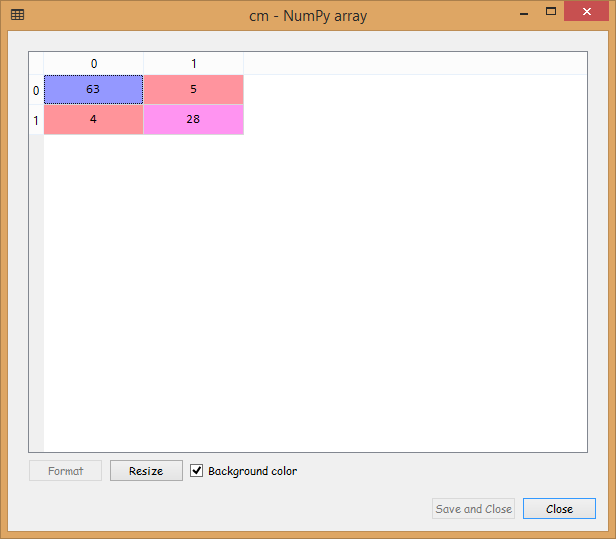
From the image given above, we can see that we have only nine incorrect predictions, which is quite good.

In the end, we will visualize the training set, and test set results, as we have done in the previous models. We will plot a graph that will differentiate the region, which predicts for the users who will buy the SUV from the region, which predicts the users who will not buy an SUV.  

Visualizing the Training Set results:

Here we are going to visualize the training set results. In this we will have a graphical visualization that will predict Yes for the users who will buy the SUV and No for the users who will not purchase the SUV, in the similar way as done before. 

Output:

From the output image given above, the points here are true results such that each point corresponds to each user of the Socical_Network (users in the dataset), and the region here are the predictions i.e., the red region contains all the users for which the classifier will predict the user does not purchase the SUV and green region contains all the user where the classifier predicts the user will buy an SUV.

The prediction boundary is the region limit between the red and green regions. We can clearly see we have a different prediction boundary then the previous classifiers. 

For each user, we have ten trees in our forest that predicted Yes if the user bought the SUV or NO if the user didn’t buy the SUV. In the previous decision tree model, we have only one tree that was making the prediction, but in the existing model, we have ten trees. After the ten trees make the predictions, they then undergo the majority voting. And so, the random forest makes the predictions Yes or No based on the majority of votes.

We can see most of the red, as well as green users, are well classified in the red region and green region, respectively. Since it is a training set, we have very few incorrect predictions.  In the next step, we will see if this Overfitting issue compromises the test set result or not.

Visualizing the Test Set results:

Now we will visualize the same for the test set.

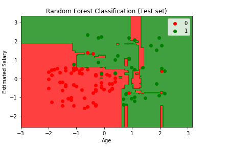
From the above output image, we can see that it is a case of Overfitting, as the red region was made to catch the red users who didn’t buy the SUV, and the green region was meant for the green users who purchased the SUV. But unfortunately, the red region is containing some of the users who bought the SUV, and the green region includes the user who didn’t purchase the SUV.

The model learned how to classify the training set, but it couldn’t make it for new observations. So, from this, it can be concluded among all the classifiers that we studied so far, the Kernel SVM classifier, and the Naïve Bayes classifier gives the most promising result, as they have a smooth curved prediction boundary that was catching correct users in the right region. Also, there was no such issue of Overfitting as it occurred in the current model while predicting new users in the test set.

Random Forest algorithm Application.

The random algorithm used in wide varieties of applications. In this article, we are going to address a few of them.

Below are some of the applications where the random forest algorithm is widely used.

1. 1. Banking
2. 2. Medicine
3. 3. Stock Market
4. 4. E-commerce

Let’s begin with the banking sector.

1.Banking:

In the banking sector, a random forest algorithm widely used in two main applications. These are for finding loyal customers and finding fraud customers.

The loyal customer means not the customer who pays well, but also the customer who can take the huge amount as loan and pays the loan interest properly to the bank. As the growth of the bank purely depends on loyal customers. The bank customer’s data is highly analyzed to find the pattern for the loyal customer based on the customer details.

In the same way, there is a need to identify the customer who is not profitable for the bank, like taking the loan and paying the loan interest properly or find outlier customers. If the bank can identify these kinds of customers before giving the loan to the customer.  Banks will get a chance to not approve the loan to these kinds of customers. In this case, a random forest algorithm is also used to identify the customers who are not profitable for the bank.

2.Medicine

In the medicine field, a random forest algorithm is used to identify the correct combination of the components to validate the medicine. Random forest algorithms are also helpful for identifying the disease by analyzing the patient’s medical records.

3.Stock Market

In the stock market, a random forest algorithm used to identify the stock behavior as well as the expected loss or profit by purchasing the particular stock.

4.E-commerce

In e-commerce, the random forest used only in the small segment of the recommendation engine for identifying the likely hood of customers liking the recommended products based on similar kinds of customers.

Running a random forest algorithm on a very large dataset requires high-end GPU systems. If you are not having any GPU system. You can always run the machine learning models on a cloud-hosted desktop. You can use a cloud desktop online platform to run high-end machine learning models from sitting in any corner of the world.

Advantages of Random Forest algorithm.

• For applications in classification problems, Random Forest algorithm will avoid the overfitting problem
• For both classification and regression task, the same random forest algorithm can be used
• The Random Forest algorithm can be used for identifying the most important features from the training dataset, in other words, feature engineering.

Disadvantages of Random Forest

Although random forest can be used for both classification and regression tasks, it is not more suitable for Regression tasks